Count Upon Security

[This is my second post on a series of articles that I would like to cover different tools and techniques to perform file system forensics of a Windows system. The first article was about acquiring a disk image in Expert Witness Format and then mount it using the SIFT workstation. The below one will be about processing the disk image and creating a timeline from the NTFS metadata. LR]

After evidence acquisition, you normally start your forensics analysis and investigation by doing a timeline analysis. This is a crucial step and very useful because it includes information on when files were modified, accessed, changed and created in a human readable format, known as MAC time evidence. This activity helps finding the particular time an event took place and in which order. Different techniques and tools exist to create timelines. In recent years an approach known as super timeline is very popular due to ability to bring together different sources of data. However, in this article we will focus on creating a timeline from a single source. The Master File Table file.

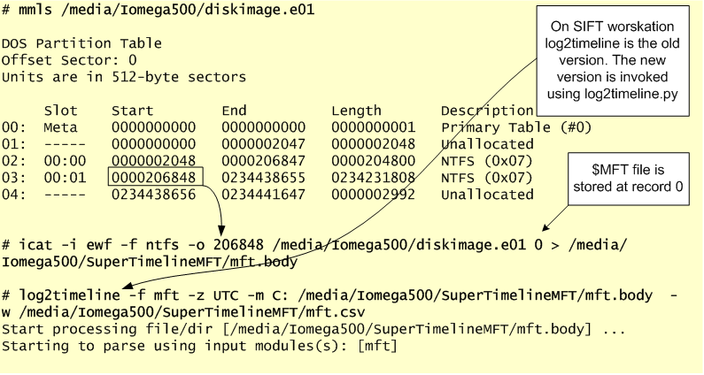
Before we move to the hand-on exercise let’s review some concepts behind the Master File Table. The Master File Table is a special system file that resides on the root of every NTFS partition. This file contains a wealth of forensic evidence. The file is named $MFT and is not accessible via user mode API’s but can been seen when you have raw access to the disk e.g, forensic image. This special file contains entries for every file and directory including itself. As written by Brian Carrier the MFT is the heart of NTFS. Each entry of the $MFT contains a series of attributes about a file, directory  and indicates where it resides on the physical disk and if is active or inactive. The active/inactive attribute is the flag that tracks deleted files. If a file gets deleted, its MFT record becomes inactive and is ready for reuse. The size of these entries are usually 1Kb. Because each record doesn’t fill 1Kb each entry contains an attribute stating if  contains resident data or not. Due to file system optimization, NTFS might store files directly on MFT records. A good example of this are Internet cookie files.  Microsoft reserves the first 16 MFT entries for special metadata files. These entries point to a special file that begins with $. The $Bitmap and $LogFile are examples of such files. A list of the first MFT entries are shown in the below picture. As well, it shows how to read the MFT record of a disk image on SIFT workstation using istat. The 0 at the end of the command is the record number you want to read for this partition that starts at offset 206848. The record 0 is the $MFT file itself.

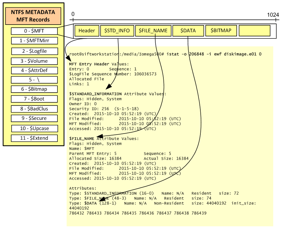
Each record contains a set of attributes. Some of the most important attributes in a MFT entry are the $STANDART_INFORMATION, $FILENAME and $DATA. The first two are rather important because among other things they contain the file time stamps. Each MFT entry for a given file or directory will contain 8 time stamps. 4 in the $STANDARD_INFORMATION and another 4 in the $FILENAME. These time stamps are known as MACE.

• M – Modified : When the contents of a file were last changed.
• A – Accessed : When the contents of a file were accessed/read.
• C – Created : When the file was created.
• E – Entry Modified : When the MFT record associated with the file changed.

For our exercise, this small introduction will suffice. Please see the references for great books on NTFS.

Now that we have reviewed some initial concepts on MFT let’s move to our hands-on exercise.  For this exercise we will need the SIFT workstation with our evidence mounted – this was done on previous article. Then we need a Windows machine where we will access the mounted evidence on the SIFT workstation using a network drive. Finally, we will need the Mft2Csv tool from Joakim Schicht on the Windows machine to read, parse and produce the MFT timeline.

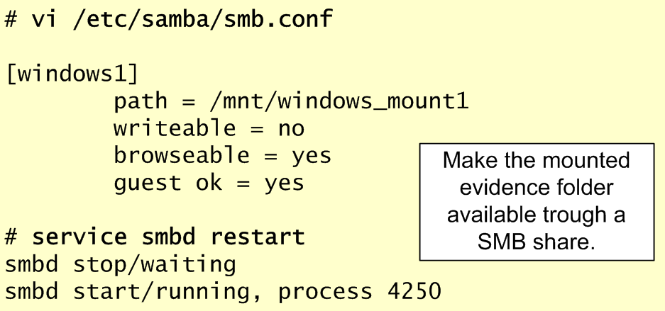
To start we share the mounted evidence on our SIFT workstation. In this case its /mnt/windows1 and was mounted on previous article. To perform this we edit the smb.conf and we add the lines as shown in the below figure. Then we restart the SMB deamon.

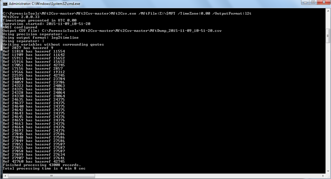
Next, from your windows machine, which needs to be in the same network segment as your SIFT workstation. you can view the shares by using the net view command. Then using the net use command you can map a drive letter. 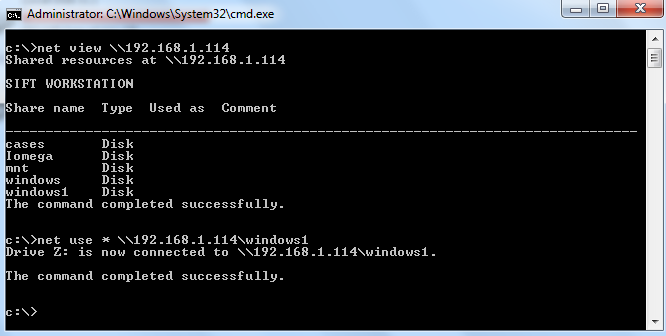With this step on our Windows machine we will have access to our mounted evidence over the Z: drive. Next step is to run Mft2Csv tool. Mft2Csv is a powerful and granular tool developed by Joakim Schicht. For those who are not familiar with Joakim Schicht, he is a brilliant engineer who has enormously contributed to the Forensics community with many powerful tools.The tool has the ability to read $MFT from a variety of sources, including live system acquisition. It runs on Windows and has GUI and CLI capabilities and needs admin rights. The tool can be downloaded from here. As we speak the last version is v2.0.0.33. In this case, we will launch it from our Windows machine. The command line parameters define from where you are reading the $MFT file and the Time zone. The output by default will be saved in a CSV format but could be saved in a log2timeline or bodyfile. If you are familiar with the log2timeline format than you could use /OutputFormat:l2t. Below picture illustrate this step. The command executed is Mft2Csv.exe /MftFile:Z:\$MFT /TimeZone:0.00 /OutputFormat:l2t 
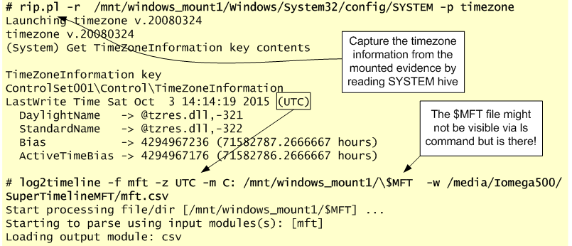
  When the command is finished you can open the timeline in Excel or copy it to SIFT workstation and use grep, awk and sed to review the entries. Another approach to create a timeline of the MFT metadata is using an old version of log2timeline which is still available on the SIFT workstation.  This old version has a MFT parser. You can use log2timeline directly on the mounted evidence. First we capture the Time Zone information from the mounted evidence using Registry Ripper – which we will cover on another post. Then we run log2timeline with -f MFT suffix to read and parse the $MFT file. The -z defines the time zone and the -m is a marker that will show prepended to the output of the filenames.

Or if you don’t have the evidence mounted you can export the $MFT using icat from TheSleuthKit.

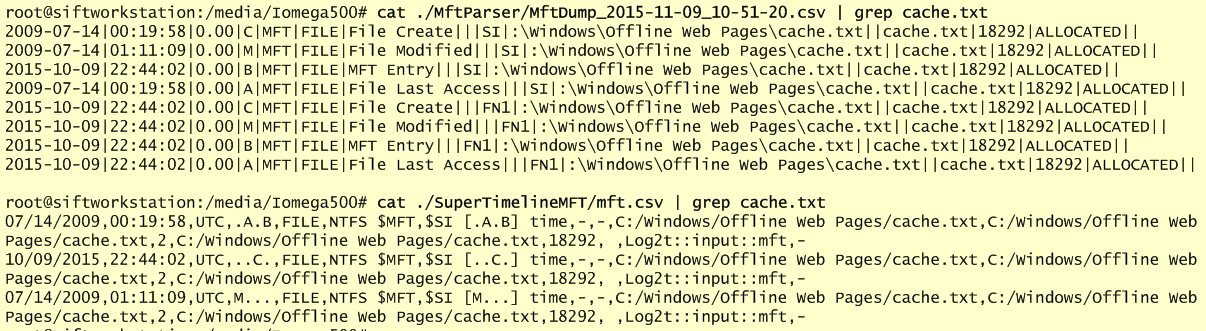
Below picture illustrates the output of both tools using the l2t format.  In this case the cache.txt is an executable file part of a system that has been compromised with w32.morto worm.

That’s it! In this article we reviewed some introductory concepts about the Master File Table and we used Mft2Csv and Log2timeline to read, parse and create a timeline of it. The techniques and tools are not new. However, they are relevant and used in today’s digital forensic analysis. Next step, review more NTFS metadata.

References:

https://github.com/jschicht/Mft2Csv/wiki/Mft2Csv
Windows Internals, Sixth Edition, Part 2 By: Mark E. Russinovich, David A. Solomon, and Alex Ionescu
File System Forensic Analysis By: Brian Carrier
SANS 508 – Advanced Computer Forensics and Incident Response