This article is a quick exercise and a small introduction to the world of Linux forensics. Below, I perform a series of steps in order to analyze a disk that was obtained from a compromised system that was running a Red Hat operating system. I start by recognizing the file system, mounting the different partitions, creating a super timeline and a file system timeline. I also take a quick look at the artifacts and then unmount the different partitions. The process of how to obtain the disk will be skipped but here are some old but good notes on how to obtain a disk image from a VMware ESX host.
When obtaining the different disk files from the ESX host, you will need the VMDK files. Then you move them to your Lab which could be simple as your laptop running a VM with SIFT workstation. To analyze the VMDK files you could use the “libvmdk-utils” package that contain tools to access data store in VMDK files. However, another approach would be to convert the VMDK file format into RAW format. In this way, it will be easier to run the different tools such as the tools from The Sleuth Kit – which will be heavily used – against the image. To perform the conversion, you could use the QEMU disk image utility. The picture below shows this step.

Following that, you could list the partition table from the disk image and obtain information about where each partition starts (sectors) using the “mmls” utility. Then, use the starting sector and query the details associated with the file system using the “fsstat” utility. As you could see in the image, the “mmls” and “fsstat” utilities are able to identify the first partition “/boot” which is of type 0x83 (ext4). However, “fsstat” does not recognize the second partition that starts on sector 1050624.

This is due to the fact that this partition is of type 0x8e (Logical Volume Manager). Nowadays, many Linux distributions use LVM (Logical Volume Manager) scheme as default. The LVM uses an abstraction layer that allows a hard drive or a set of hard drives to be allocated to a physical volume. The physical volumes are combined into logical volume groups which by its turn can be divided into logical volumes which have mount points and have a file system type like ext4.
With the “dd” utility you could easily see that you are in the presence of LVM2 volumes. To make them usable for our different forensic tools we will need to create device maps from the LVM partition table. To perform this operation, we start with “kpartx” which will automate the creation of the partition devices by creating loopback devices and mapping them. Then, we use the different utilities that manage LVM volumes such as “pvs”, “vgscan” abd “vgchange”. The figure below illustrates the necessary steps to perform this operation.

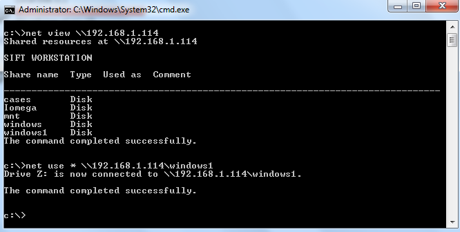
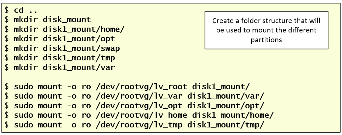
After activating the LVM volume group, we have six devices that map to six mount points that make the file system structure for this disk. Next step, mount the different volumes as read-only as we would mount a normal device for forensic analysis. For this is important to create a folder structure that will match the partition scheme.
After mounting the disk, you normally start your forensics analysis and investigation by creating a timeline. This is a crucial step and very useful because it includes information about files that were modified, accessed, changed and created in a human readable format, known as MAC time evidence (Modified, Accessed, Changed). This activity helps finding the particular time an event took place and in which order.
Before we create our timeline, noteworthy, that on Linux file systems like ext2 and ext3 there is no timestamp about the creation/birth time of a file. There are only 3 timestamps. The creation timestamp was introduced on ext4. The book “The Forensic Discovery 1st Edition”from Dan Farmer and Wietse Venema outlines the different timestamps:
- Last Modification time. For directories, the last time an entry was added, renamed or removed. For other file types, the last time the file was written to.
- Last Access (read) time. For directories, the last time it was searched. For other file types, the last time the file was read.
- Last status Change. Examples of status change are: change of owner, change of access permission, change of hard link count, or an explicit change of any of the MACtimes.
- Deletion time. Ext2fs and Ext3fs record the time a file was deleted in the dtime stamp.the filesystem layer but not all tools support it.
- Creation time: Ext4fs records the time the file was created in crtime stamp but not all tools support it.
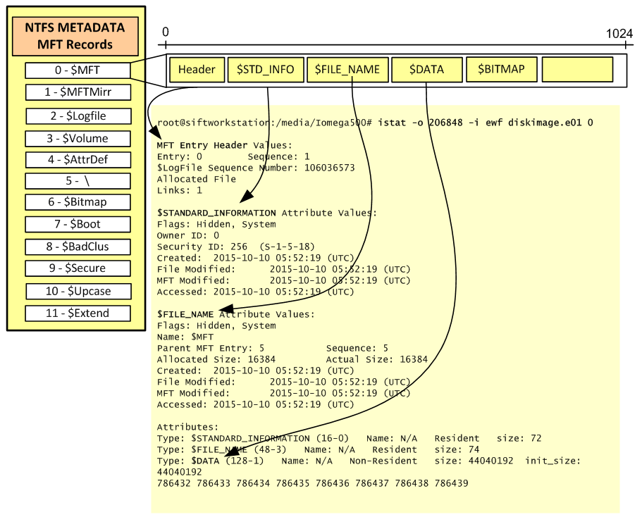
The different timestamps are stored in the metadata contained in the inodes. Inodes are the equivalent of MFT entry number on a Windows world. One way to read the file metadata on a Linux system is to first get the inode number using, for example, the command “ls -i file” and then you use “istat” against the partition device and specify the inode number. This will show you the different metadata attributes which include the time stamps, the file size, owners group and user id, permissions and the blocks that contains the actual data.
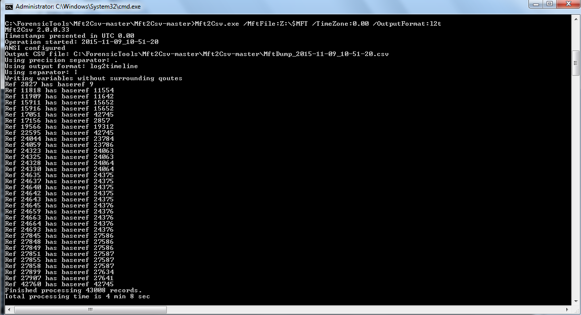
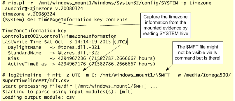
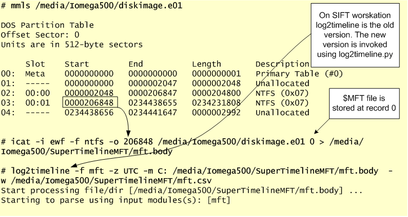
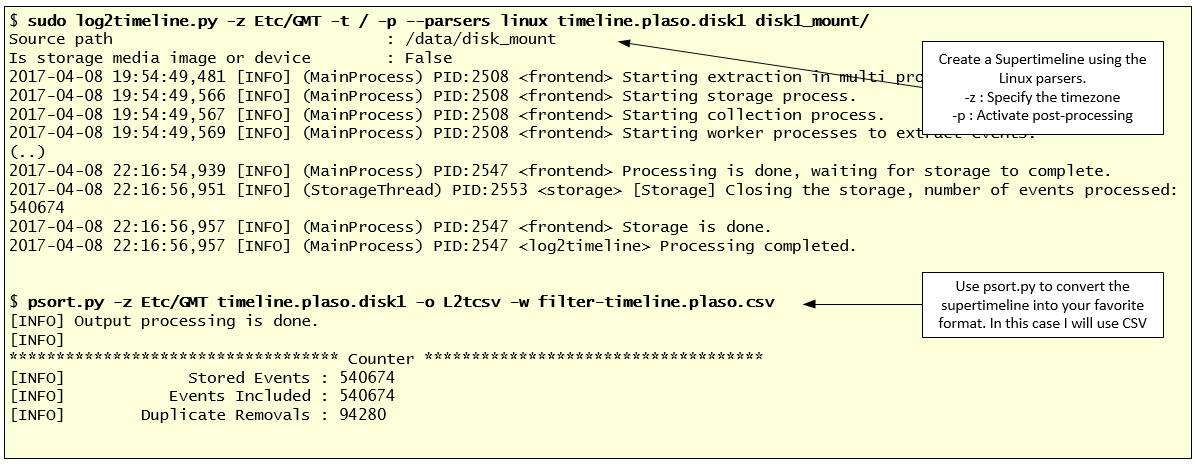
Ok, so, let’s start by creating a super timeline. We will use Plaso to create it. For contextualization Plaso is a Python-based rewrite of the Perl-based log2timeline initially created by Kristinn Gudjonsson and enhanced by others. The creation of a super timeline is an easy process and it applies to different operating systems. However, the interpretation is hard. The last version of Plaso engine is able to parse the EXT version 4 and also parse different type of artifacts such as syslog messages, audit, utmp and others. To create the Super timeline we will launch log2timeline against the mounted disk folder and use the Linux parsers. This process will take some time and when its finished you will have a timeline with the different artifacts in plaso database format. Then you can convert them to CSV format using “psort.py” utility. The figure below outlines the steps necessary to perform this operation.
Before you start looking at the super timeline which combines different artifacts, you can also create a traditional timeline for the ext file system layer containing data about allocated and deleted files and unallocated inodes. This is done is two steps. First you generate a body file using “fls” tool from TSK. Then you use “mactime” to sort its contents and present the results in human readable format. You can perform this operation against each one of the device maps that were created with “kpartx”. For sake of brevity the image below only shows this step for the “/” partition. You will need to do it for each one of the other mapped devices.

Before we start the analysis, is important to mention that on Linux systems there is a wide range of files and logs that would be relevant for an investigation. The amount of data available to collect and investigate might vary depending on the configured settings and also on the function/role performed by the system. Also, the different flavors of Linux operating systems follow a filesystem structure that arranges the different files and directories in a common standard. This is known as the Filesystem Hierarchy Standart (FHS) and is maintained here. Its beneficial to be familiar with this structure in order to spot anomalies. There would be too much things to cover in terms of things to look but one thing you might want to run is the “chkrootkit” tool against the mounted disk. Chrootkit is a collection of scripts created by Nelson Murilo and Klaus Steding-Jessen that allow you to check the disk for presence of any known kernel-mode and user-mode rootkits. The last version is 0.52 and contains an extensive list of known bad files.
Now, with the supertimeline and timeline produced we can start the analysis. In this case, we go directly to timeline analysis and we have a hint that something might have happened in the first days of April.
During the analysis, it helps to be meticulous, patience and it facilitates if you have comprehensive file systems and operating system artifacts knowledge. One thing that helps the analysis of a (super)timeline is to have some kind of lead about when the event did happen. In this case, we got a hint that something might have happened in the beginning of April. With this information, we start to reduce the time frame of the (super)timeline and narrowing it down. Essentially, we will be looking for artifacts of interest that have a temporal proximity with the date. The goal is to be able to recreate what happen based on the different artifacts.
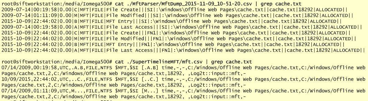
After back and forth with the timelines, we found some suspicious activity. The figure below illustrates the timeline output that was produced using “fls” and “mactime”. Someone deleted a folder named “/tmp/k” and renamed common binaries such as “ping” and “ls” and files with the same name were placed in the “/usr/bin” folder.

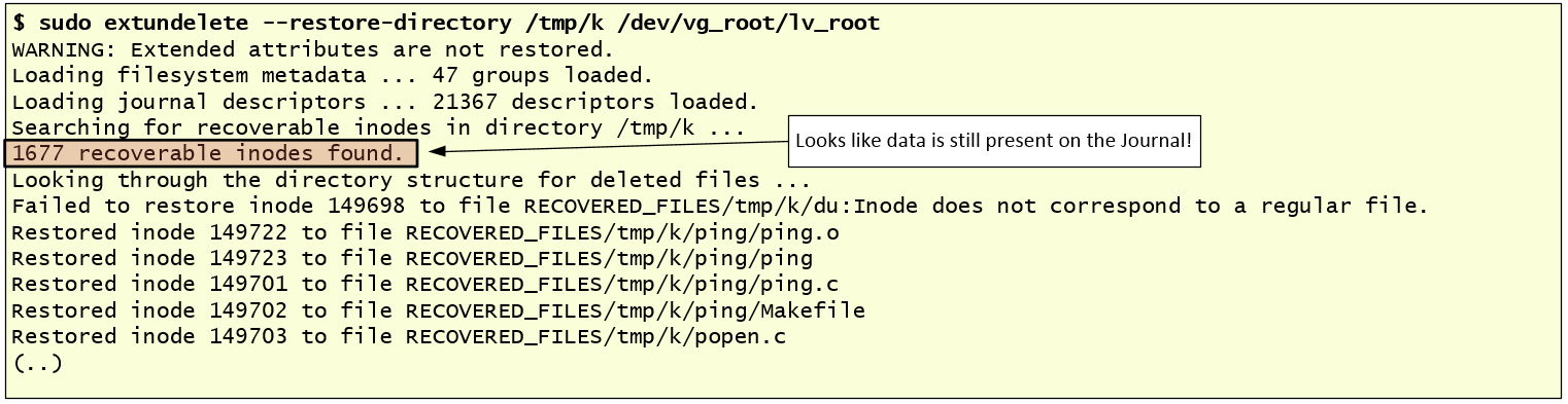
This needs to be looked further. Looking at the timeline we can see that the output of “fls” shows that the entry has been deleted. Because the inode wasn’t reallocated we can try to see if a backup of the file still resides in the journaling. The journaling concept was introduced on ext3 file system. On ext4, by default, journaling is enabled and uses the mode “data=ordered”. You can see the different modes here. In this case, we could also check the options used to mount the file system. To do this just look at “/etc/fstab”. In this case we could see that the defaults were used. This means we might have a chance of recovering data from deleted files in case the gap between the time when the directory was deleted and the image was obtained is short. File system journaling is a complex topic but well explained in books like “File system forensics” from Brian Carrier. This SANS GCFA paper from Gregorio Narváez also covers it well. One way you could attempt to recover deleted data is using the tool “extundelete”. The image below shows this step.
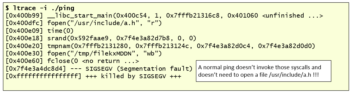
The recovered files would be very useful to understand more about what happened and further help the investigation. We can compute the files MD5’s, verify its contents and if they are known to the NSLR database or Virustotal. If it’s a binary we can do strings against the binary and deduce functionality with tools like “objdump” and “readelf”. Moving on, we also obtain and look at the different files that were created on “/usr/sbin” as seen in the timeline. Checking its MD5, we found that they are legitimate operating system files distributed with Red Hat. However, the files in “/bin” folder such as “ping” and “ls” are not, and they match the MD5 of the files recovered from “/tmp/k”. Because some of the files are ELF binaries, we copy them to an isolated system in order to perform quick analysis. The topic of Linux ELF binary analysis would be for other time but we can easily launch the binary using “ltrace -i” and “strace -i” which will intercept and record the different function/system calls. Looking at the output we can easily spot that something is wrong. This binary doesn’t look the normal “ping” command, It calls the fopen() function to read the file “/usr/include/a.h” and writes to a file in /tmp folder where the name is generated with tmpnam(). Finally, it generates a segmentation fault. The figure below shows this behavior.
Provided with this information, we go back and see that this file “/usr/include/a.h” was modified moments before the file “ping” was moved/deleted. So, we can check when this “a.h” file was created – new timestamp of ext4 file system – using the “stat” command. By default, the “stat” doesn’t show the crtime timestamp but you can use it in conjunction with “debugfs” to get it. We also checked that the contents of this strange file are gibberish.

So, now we know that someone created this “a.h” file on April 8, 2017 at 16:34 and we were able to recover several other files that were deleted. In addition we found that some system binaries seem to be misplaced and at least the “ping” command expects to read from something from this “a.h” file. With this information we go back and look at the super timeline in order to find other events that might have happened around this time. As I did mention, super timeline is able to parse different artifacts from Linux operating system. In this case, after some cleanup we could see that we have artifacts from audit.log and WTMP at the time of interest. The Linux audit.log tracks security-relevant information on Red Hat systems. Based on pre-configured rules, Audit daemon generates log entries to record as much information about the events that are happening on your system as possible. The WTMP records information about the logins and logouts to the system.
The logs shows that someone logged into the system from the IP 213.30.114.42 (fake IP) using root credentials moments before the file “a.h” was created and the “ping” and “ls” binaries misplaced.

And now we have a network indicator. Next step we would be to start looking at our proxy and firewall logs for traces about that IP address. In parallel, we could continue our timeline analysis to find additional artifacts of interest and also perform in-depth binary analysis of the files found, create IOC’s and, for example, Yara signatures which will help find more compromised systems in the environment.
That’s it for today. After you finish the analysis and forensic work you can umount the partitions, deactivate the volume group and delete the device mappers. The below picture shows this steps.

Linux forensics is a different and fascinating world compared with Microsoft Windows forensics. The interesting part (investigation) is to get familiar with Linux system artifacts. Install a pristine Linux system, obtain the disk and look at the different artifacts. Then compromise the machine using some tool/exploit and obtain the disk and analyze it again. This allows you to get practice. Practice these kind of skills, share your experiences, get feedback, repeat the practice, and improve until you are satisfied with your performance. If you want to look further into this topic, you can read “The Law Enforcement and Forensic Examiner’s Introduction to Linux” written by Barry J. Grundy. This is not being updated anymore but is a good overview. In addition, Hal Pomeranz has several presentations here and a series of articles written in the SANS blog, specially the 5 articles written about EXT4.
References:
Carrier, Brian (2005) File System Forensic Analysis
Nikkel, Bruce (2016) Practical Forensic Imaging