FireEye Endpoint Security (HX) – Supplementary Tools

Today I am going to write a few notes about tools that should be part of your toolkit in case you use FireEye Endpoint Security product a.k.a. as HX. If you don’t use FireEye HX, this post likely has no interest for you.

I tend to use HX when performing large scale Enterprise Forensics and Incident Response. I also tend to see HX or other EDR solutions on organizations with mature security operations that use such technology to increase endpoint visibility and improve their capabilities to detect and respond to threats on the endpoints. HX is very powerful,  feature rich but like many EDR products it tends to be designed for more seasoned incident responders with specialized skill set. HX can be used in the realm of protection, detection, and response. Today’s notes are primarily focused on two things: Increase awareness about tools that will help augment HX capability to detect attacks; Increase awareness about tools that will help the analyst ability to work with the results. Goal is to improve threat detection and ability to analyze the results therefore increase the effectiveness of your product and maximize the outcome of your investigations.

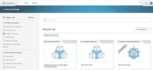
FireEye makes available a website named fireeye.market where one can download apps that extend the functionality of existing products. If you are a FireEye customer you likely have seen this before. For this post I’m looking at the Endpoint Security apps that might extend the functionality of the HX or enhance the analyst ability to perform the work faster/better.  On the FireEye Market website there are a few things that are freeware and can be downloaded without subscription. Others may require a subscription. One of the main freeware tools is the IOC Editor. Let’s briefly go over some of the things that will be useful.

Indicators of Compromise (IOC) Editor is a free tool for Windows that provides an interface for managing data and manipulating the logical structures of IOCs. IOCs are XML documents that help incident responders capture diverse information about threats, including attributes of malicious files, characteristics of registry changes, artifacts in memory, etc.  There are two versions of IOC editor in the website. We want the IOC 1.1 editor version 3.2. The installation file Mandiant IOCe.msi can be downloaded from here  https://fireeye.market/apps/211404 . The archive is IOCe-3.2.0-Signed.msi.zip (3EE56F400B4D8F7E53858359EDA9487C). This version brings updated IOC terms that allow us to create IOCs for HX real-time alerting and for searching the contents of the HX event buffer (ring buffer). Note that Redline does not support IOC 1.1. If you are a developer or interested in the details IOC 1.1 specification you can look here https://github.com/mandiant/OpenIOC_1.1. This schema is what Mandiant services uses internally to extend functionality of IOC Editor and support new and extended terms. The IOC editor contains two main set of terms: On one hand you have the terms that can be used to search for historical artefacts (Sweep) and on the other hand you have the terms that can be used to search event buffer (Real-Time) or generate real time alerts. All terms are created with a set of conditions and logic needed to describe and codify the forensic artefacts.

OpenIOC2HXIOC

When you use IOC editor to create, edit, maintain your Real-Time IOCs you need to upload them to HX either for testing or to be on released on production. One way to accomplish this is to use the Python script that takes IOCs as input and uploads them into HX to be used on Real Time alerting. This script can be downloaded from https://fireeye.market/apps/213060. You will need Python and a HX user account with API rights because the script takes advantage of the HX API to perform the work.

HXTOOL

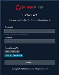
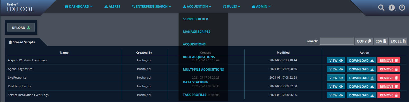
HXTool, originally created by Henrik Olsson in 2016, is a web-based, opensource, standalone tool written in python. that can be used with HX. HXTool provides additional features not directly available in the product GUI by leveraging FireEye Endpoint Security’s rich API. Since the code now is open source, this tool is an excellent example of how you can develop applications utilizing the Endpoint Security REST API. It is available in FireEye’s public GitHub at https://github.com/fireeye/HXTool.

After installation, open a webbrowser and point it to localhost on port 8080. In the HXTool create a new profile with the IP address and port of the HX controller. Then connect with a user that has API Admin rights and was previously created in the HX management interface. There are many features in HX tool but the ability to use Script Builder to create audit scripts allows you fully leverage the potential of HX. After you create a script you run Sweeps using the bulk-acquisition method. The Sweeps can be used to perform enterprise forensics at scale or to look for real time data stored in the ring buffer of the endpoints. Nonetheless, you can use HXTool to perform stack analysis, enterprise searches based on OpenIOC 1.1, create, and maintain the Real-Time indicators, etc.

$ git clone https://github.com/fireeye/HXTool
Cloning into 'HXTool'...
remote: Enumerating objects: 6401, done.
remote: Counting objects: 100% (90/90), done.
remote: Compressing objects: 100% (70/70), done.
remote: Total 6401 (delta 39), reused 55 (delta 20), pack-reused 6311
Receiving objects: 100% (6401/6401), 14.64 MiB | 5.08 MiB/s, done.
Resolving deltas: 100% (4337/4337), done.  
$cd HXTool/   $ pip install -r requirements.txt --user
(..)
Installing collected packages: itsdangerous, MarkupSafe, Jinja2, click, Werkzeug, flask, pycryptodome, tinydb, six, python-dateutil, numpy, pytz, pandas Successfully installed Jinja2-2.11.2 MarkupSafe-1.1.1 Werkzeug-1.0.1 click-7.1.2 flask-1.1.2 itsdangerous-1.1.0 numpy-1.16.6 pandas-0.24.2 pycryptodome-3.9.7 python-dateutil-2.8.1 pytz-2020.1 six-1.15.0 tinydb-3.15.2    
$ python3 hxtool.py
(..)
[2020-06-02 01:39:41,497] {hxtool} {MainThread} INFO - Application starting
[2020-06-02 01:39:41,501] {hxtool} {MainThread} INFO - Application is running. Please point your browser to https://0.0.0.0:8080. Press Ctrl+C/Ctrl+Break to exit.  
* Serving Flask app "hxtool" (lazy loading)  
* Environment: production   
WARNING: This is a development server. Do not use it in a production deployment.    Use a production WSGI server instead.  
* Debug mode: off

Supplementary  IOCs

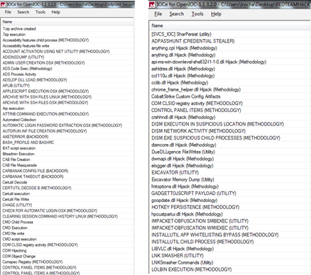
In the FireEye market website, there are a set of FireEye released Real-Time IOCs designed to supplement FireEye Endpoint Security’s production indicators. They were created for environment-specific detection and testing, like tests based on MITRE’s ATT&CK framework. Most of these IOCs will require substantial tuning to use in a production environment. They need to be customized for your environment and should not be uploaded in bulk. This set contains more than 400 IOCs and can be obtained from https://fireeye.market/apps/234563

FireEye Red Team IOCs.  Last December as result of an incident, FireEye released a set of IOCs to detect FireEye Red Team tools. These IOCs empower the community to detect these tools and are available in different formats including OpenIOC, Yara, Snort, and ClamAV. There are more than 80 IOCs in OpenIOC format and can be downloaded from https://github.com/fireeye/red_team_tool_countermeasures

The first set of IOCs are very broad and need to be customized for a particular environment but they offer a starting point for security teams to test and get familiar with the process. The lifecycle of designing, building, deploying, and adopting IOCs is part of the Security monitoring and/or Incident Response capability where well trained and well equipped personnel alongside with consistent and well defined process come into play. If you want to be able to run sophisticated threat hunting missions you first should be able to understand the threat, understand the indicators that help you identify the threat in your network and then you can create and maintain IOCs that may represent that threat. The second set of IOCs are overall very good but some of them need tunning specially the LOLBINs and the suspicious DLL executions.

GOAUDITPARSER

So, by now, with the things that were covered, you have a set of IOCs that you uploaded to HX using the OpenIOC2HXIOC script and you used the HXTool to Sweep your environment to look for threats or you used them to generate Real-Time alerts. But how to analyze the results? Traditionally you likely used the HX GUI or downloaded the data and used Redline. However, we can now use some other technique.  Daniel Pany just recently open sourced GoAuditParser. A versatile and customizable tool to help analysts work with FireEye Endpoint Security product (HX) to extract, parse and timeline XML audit data. People have used Redline to parse and create a timeline of the data acquired with HX but using this tool an analyst may be able to improve his ability to perform analysis on the data at scale obtained via HX. The compiled builds of the tool can be downloaded from https://github.com/fireeye/goauditparser/releases/tag/v1.0.0. Danny has published extensive documentation on how to use the tool on GitHub.

GAP_4_1_4

That’s it for today. If you use HX you can now improve your investigation methods using the mentioned tools. Consider and think about the following 3 steps:

  • Based on leads or alerts you collect Live Response data
    • Use HXTool Script Builder to create a script to acquire Live Response Data
    • Use HXTool to run a Bulk Acquisition to run the acquisitions of Live Response data
    • Download the Live Response Acquisition using HXTool
  • Analyze results & develop timeline
    • Use GoAuditParser to extract, parse and timeline the results.
    • Perform the forensic investigation by interpreting the results
    • Use your favorite tool to create a timeline (likely Excel)
  • Design, build, deploy and adopt Real-Time IOCs and Sweep IOCs
    • Use IOC editor to build IOCs that represent your findings
    • Use IOC editor to create IOCs for both Sweeps and Real-Time
    • Deploy Real-Time IOCs using OpenIOC2HXIOC
    • Create Sweeps with HXTool using Script Builder, Job Filters in conjunction with IOCs to filter results and BulkAcquistions.
  • Repeat

Hopefully this short summary increases the awareness on how to use HX more efficiently. It also serves to capture a perspective on how to use HX because you can use such tools to handle real security incidents and intrusions at enterprise level.

References:

Endpoint Security Server User Guide Release 5.0.2
Endpoint Security Server System Administration Guide Release 5.0.2
IOC Editor 2.2.0.0 User Guide


Tagged , , , , ,

Notes on Linux Memory Analysis – LiME, Volatility and LKM’s

[The post below contains some notes I wrote about Linux memory forensics using LiME and Volatility to analyze a Red Hat 6.10 memory capture infected with Diaphormine and Reptile, two known Linux Kernel Module rootkits.]

Back in 2011, Joe Sylve, Lodovico, Marziale, Andrew Case, and Golden G. Richard published a research paper on acquiring and analyzing memory from Android devices “Acquisition and analysis of volatile memory from android devices” [1]. At Shmoocon 2012, Joy Sylve gave a presentation titled “Android Mind Reading: Memory Acquisition and Analysis with DMD and Volatility“[2]. This work was the precursor of Linux Memory Extractor aka LiME [3]. LiME is an open source tool, created by Joy Sylve, that allows incident responders, investigators and others to acquire a memory sample from a live Linux system.

Some years before, The Volatility Framework was developed based on the research that was done by AAron Walters and Nick Petroni on Volatools [4] and FATkit [5]. The first release of the Volatility Framework was released in 2007. In 2008 the volatility team won the DFRWS challenge [6] and the new features were added to Volatility 1.3.  At the moment, Volatility is a powerful, modular and feature rich framework that combines a number of tools to perform memory analysis. The framework is written in Python and allows plugins to be easily added in order to add features. Nowadays it is on version 2.6.1 and version 3 is due this month. It supports a variety of operating systems. To analyze memory captures from Linux systems, Andrew Case, in 2011 [7], introduced several techniques into the Volatility framework in order to analyze Linux memory samples. Since then, new plugins have been introduced and different kernel versions are supported. At the moment there are 69 Linux plugins available.

Worth to mention that Michael Hale Ligh, Andrew Case, Jamie Levy, AAron Walters wrote the book “The Art of Memory Forensics Detecting Malware and Threats in Windows, Linux, and Mac Memory” that was published by Wiley in 2014 and is a reference book in this subject.

LiME works by loading a kernel driver on the live system and dump the memory capture to disk or network. The only catch is that the loadable kernel module needs to be compiled for the exact version of the kernel of the target system. Volatility is then be able to interpret this memory capture, but it needs a profile that matches the system from where the memory was acquired. Building a Volatility profile is straightforward, but it requires kernel’s data structures and debug symbols obtained for the exact kernel version of the target system obtained using the dwardfump utility.  This means that if you want to acquire a memory capture from a system in an enterprise, the incident response team will need to transfer LiME and Volatility code to the system and compile it in order to create the required files. Sometimes the target system won’t have the necessary dependencies and additional packages will need to be installed such as compilers, DWARF libraries, ELF utilities, Kernel headers, etc. This is a sensible step from a forensic standpoint. Hal Pomeranz, experienced forensics professional, has a few comments about this on the readme file from his Linux Memory Grabber utility [8].

In an ideal world all the requirements necessary to have LiME kernel module and Volatility profile for all your Linux kernel versions will be done in advance. This can be done and should be done during the preparation phase [9] of your incident response process. This phase/step is when incident response team prepares and trains for an incident. One thing that can be done is creating LiME modules and Volaility profiles for the Kernel versions of the systems that are running in production. This can be done directly on the system or on a pre-production system. Of course, I can tell you that based on my experience, this hardly happens. Its more common the case when an incident happens i.e., an attacker used a Linux system in an enterprise environment as a staging environment or used it to achieve persistence or use it to pivot into other network segments, there are no LiME kernel modules or Volatility profiles for the compromised system. Yes, the incident response team acquires live response data or a forensic image of the disk but the acquisition of memory can aid the investigation efforts.

During enterprise incident response its common to come across the need to analyze commercial Linux systems such as Red Hat that are running business applications. In this article I will be looking at a RedHat Enterprise Linux Server release 6.10 with code name Santiago.

The following illustration shows the steps for compiling LiME on the target system. I start by checking the Kernel version following by installing the necessary dependencies on this particular system. The LiME package can be retrieved from GitHub and can be made available to the target system using removable media, a network file share, or by copying into the system. Compiling LiME is an easy step.

Next step is to run LiME with the insmod command. This step will acquire a memory sample in LiME format and in this case I also told LiME to produce a hash of the acquired memory sample. As an example the memory capture is written to disk but in a real incident is should be written to a network share, removable media sent via the network. Finally, you can remove the module with rmmod.

After that, we need a Volatility profile for the Linux kernel version we are dealing with. On this version of RedHat I could not find a RPM for Libdwarf that contained the Dwarf tools. I had to get the source code from GitHub and transfer it to the system and compile it. Then, with the dependencies met I could compile and make the dwarf module.

Finally, I acquired the system-map file and zipped it together with module.dwarf. This zip file needs to be placed in the volatility profiles folder or you can place it on a different folder and specify it in the command line.

Now that I have a profile for the Linux system that I can try different Volatility plugins. In this particular case I was interested in determining what I could observe when looking with Volatility on a memory capture from the system after it has been backdoored with publicly available rootkits. There are several Volatility plugins for Volatility that can help identifying rootkits [10]. Let’s review three that might help with rootkits that leverage Linux Kernel Modules..

The linux_check_modules plugin. This plugin will look for kernel loadable modules that are not listed under /proc/module but still appear under /sysfs/module and will show the discrepancies. There is also the linux_hidden_modules which will look at the kernel memory region where modules are allocated and scans for module structures. Modules appearing with this plugin might indicate they were released but still laying in memory or they are hiding.

The linux_check_syscall plugin. This plugin will check if the sys_call_table has been modified. It lists all syscall handler function pointers listed in the sys_call_table array and it compares them with the address specified in the Kernel Symbols Table. If they don’t match, the message hook will be displayed.

The linux_check_kernel_inline plugin. This plugin will detect inline hooking. Among other things it will check if the prologue of specific functions in the kernel contains assembly instructions like JMP, CALL or RET. A match will display a message about the function that is being hooked.

In terms of Rootkits that leverage Loadable Kernel Modules I will look into Diamorphine [11] and Reptile [12]. Essentially, infecting the Red Hat system with the rootkit and capture a memory sample.

Let’s start with Diamorphine. Written by Victor Mello is a kernel rootkit written in C that supports Linux Kernels 2.6.x/3.x/4.x. It can hide processes, files and directories. It works by hooking the sys_call_table, more specifically it hooks the kill, getdents and getdents64 syscall handler addresses, making them point to the Diaphormine code. After loading into memory, the LKM module won’t be visible in /proc/modules but is still visible under /sys/module.

The following illustration shows, as an example, the Reptile installation on a Red Hat 6.10 system. It also shows that after the insertion of the malicious module into the Kernel, it doesn’t appear under /proc/modules. There is also a step on hiding a PID referent to bash process.

Following the previous steps, another memory sample was captured, and I ran the linux_check_modules Volatility plugin. As we could see, the plugin was able to find the Reptile module because he was still visible under /sysfs/module. We could dump the module to disk using the linux_moddump (didn’t worked for me at the time I tried it) and perform additional analysis in case this was something we were uncertain about. In this case I just looked at the first bytes of the module using linux_volshell plugin. The Volshell plugin was created in 2008 by Brendan Dolan-Gavitt. Following ilustration shows the usage of VolShell to print out 128 bytes in ASCII and look for interesting strings.

The other plugin worth to run is linux_check_syscall, which in this case is able to detect three hooked syscalls. Syscall 62, 78 and 217 which we can match against the syscall table from the pristine system, by looking at /proc/kallsyms, and check that the number corresponds to sys_kill, sys_getdents and sys_getdents64, respectively. Following that, and from a analysis perspective, I could use VolShell on the pristine memory dump and also on the one that has Diaphormine LKM loaded. Then I could list a few bytes in Assembly to compare and understand how good and bad looks like. In the following picture, on the left side, you can see the good sys_kill function and on the left side the bad one. Basically the syscall handler address was modified to point to the Diaphormine code.

The other rootkit that is worth to look at is Reptile. It was written by Ighor Augusto and is a feature rich rootkit with features like port knocking. It is written in C and under the hood it uses the Khook framework. You can see the presentation “Linux Kernel Rootkits Advanced Techniques” from Ilya Matveychikov and Ighor Augusto that was given during H2HC 2018 [13] conference at São Paulo, Brasil where Reptile was released. Khook, among other things, instead of hooking the sys_call_table it uses a different technique that patches a function prologue with a JMP instruction. With the Volatility linux_check_syscal plugin we can’t detect this hooking technique since the syscall handler addresses have not been modified but it can be identified with linux_check_kernel_inline. Among other things, Reptile hooks fillonedir(), filldir(), filldir64(), compat_fillonedir(), compat_filldir(), compat_filldir64(), __d_lookup(). To hide processes, it hooks tgid_iter() and next_tgid(). To hide network connections, it hooks tcp4_seq_show and udp4_seq_show.

The following illustration shows, as an example, the Reptile installation on a Red Hat 6.10 system.

After compromising a system with Reptile and acquiring a memory capture, I executed the mentioned plugins. I started with linux_hidden_modules to look for LKM structures in the Kernel Memory. Volatility was able to find the Reptile LKM. Then we could dump the module to disk and perform additional static analysis.

The other plugin executed is linux_check_inline_kernel. It was able to detect several network related functions that were patched by the Reptile code. I didn’t had time to further investigate why the Hook Address is not shown but we can get futher details with Volshell.

The following picture shows a comparison of a good tcp4_seq_show function on the left side from a memory capture of a pristine system and, on the right, it shows the same function but as we could see it has been patched to jump (JMP) to the Reptile code.

Another function that is patched by Reptile code in order to hide directories is the filleonedir. Not sure why Volatility didn’t detected this but the plugin might be easily adjustable to perform further checks and detect it. On the image below, on the left side, I used Volshell to check the function prologue on a pristine system. On the right side, we can see how the patched function looks like.

That’s it for today. In this post I shared some notes on how to use different Volatility plugins to detect known Rootkits that leverage Linux Kernel Modules. The memory capture was obtained using LiME and and instructions were given on how to acquire the memory capture and create a Volatility profile. Nothing new but practice these kind of skills, share your experiences, get feedback, repeat the practice, and improve until you are satisfied with your performance. Have fun!

[1] http://www.dfir.org/research/android-memory-analysis-DI.pdf

[2] https://www.youtube.com/watch?v=oWkOyphlmM8

[3] https://github.com/504ensicsLabs/LiME

[4] https://www.blackhat.com/presentations/bh-dc-07/Walters/Paper/bh-dc-07-Walters-WP.pdf

[5] http://4tphi.net/fatkit/papers/fatkit_journal.pdf

[6] http://volatilesystems.blogspot.com/2008/08/pyflagvolatility-team-wins-dfrws.html

[7] http://dfir.org/research/omfw.pdf

[8] https://github.com/halpomeranz/lmg

[9] https://nvlpubs.nist.gov/nistpubs/SpecialPublications/NIST.SP.800-61r2.pdf

[10] https://github.com/volatilityfoundation/volatility/wiki/Linux-Command-Reference

[11] https://github.com/m0nad/Diamorphine

[12] https://github.com/f0rb1dd3n/Reptile/

[13] https://github.com/h2hconference/2018/

References:

SANS FOR526: Advanced Memory Forensics & Threat Detection

The Art of Memory Forensics Detecting Malware and Threats in Windows, Linux, and Mac Memory

Tagged , , , , , ,

Six Years ago …

On 4th of November 2012, Count Upon Security was born. This weekend was it’s 6th anniversary!

I started this project has hobby in my spare time. I wanted to share with the IT Security community material and illustrations which I thought could be useful. Till now I’ve written 112 posts on a variety of security topics. Many with the help of good old friends. Some were short, others took weeks to write. Also 3 articles were written by Ricardo Dias and 1 by Angel Alonso. For what is worth, Akismet statistics reported that the site had 208k views and 135k visitors in 2017. In the last 5 months, due to good reasons, I didn’t have the chance to write new posts/articles. However, I really appreciate all the people who have read one or more articles or use it as reference or in some training material because it gives me incentive to continue. Hopefully, in 6 years from now, in 2024 I hope to still be here contributing to this small alley of the Internet with new content on this always evolving and fascinating industry. Stay tuned and have fun!

Digital Forensics – PlugX and Artifacts left behind

When an attacker conducts an intrusion using A, B or C technique, some of his actions leave artifact X, Y or Z behind. So, based on the scenario from the last article about PlugX, I collected a disk image and memory image from the domain controller. Over the past years I wrote several articles on how to perform acquisition, mounting and processing of such images and analyze them by creating super timelines, look at different artifacts like Event Logs, Prefetch, ShimCache, AMCache, etc., or analyze NTFS metadata or look for artifacts related to interactive sessions. Today, I’m not going to perform analysis but I’m going to list a quick overview about some of the Windows endpoint artifacts that might give us evidence about the actions that were executed in the previous scenario and help us produce a meaningful timeline. In addition, I list some tools that could be used to analyze those artifacts.

Scenario 1: The attacker placed the filename “kas.exe” on the folder “c:\PerfLogs\Admin”. Which artifacts could record evidence about this action?

  • NTFS MFT
    • Description: The Master File Table (MFT) is a special system file that resides on the root of every NTFS partition. The file is named $MFT and is not accessible via user mode API’s but can been seen when you have raw access to the disk e.g, forensic image. This special file is a hierarchical database and inside you have records that contains a series of attributes about a file, directory and indicates where it resides on the physical disk and if is active or inactive. The size of each MFT record is usually 1024-bytes. Each record contains a set of attributes. Some of the most important attributes in a MFT entry are the $STANDART_INFORMATION, $FILENAME and $DATA. The first two are rather important because among other things they contain the file time stamps. Each MFT entry for a given file or directory will contain 8 timestamps. 4 in the $STANDARD_INFORMATION and another 4 in the $FILENAME. These time stamps are known as MACE.
    • Tools: Parse and analyze it with SleuthKit originally written by Brian CarrierMFT2CSV from Joakim Schicht or PLASO/log2timeline originally created by Kristinn Gudjonsson
  • NTFS INDX Attribute
    • Description: The MFT records for directories contain a special attribute called $I30. This attribute contains information about file names and directories that are stored inside a directory. This special attribute is also known as $INDX and consists of three attributes, the $INDEX_ROOT, $INDEX_ALLOCATION and $BITMAP. So, What? Well, this attribute stores information in a B-tree data structure that keeps data sorted so the operating system can perform fast searches in order to determine if a file is present. In addition, this attribute grows to keep track of file names inside the directory. However, when you delete a file from a directory the B-tree re-balances itself but the tree node with metadata about the deleted file remains in a form of slack space until it gets reused. This means we can view the $I30 attribute contents and we might find evidence of files that once existed in a directory but are no longer there.
      Tools: o Parse it and analyze it with INDXParse from William Ballenthin or MFT2CSV from Joakim Schicht.
  • NTFS $LogFile
    • Description: NTFS has been developed over years with many features in mind, one being data recovery. One of the features used by NTFS to perform data recovery is the Journaling. The NTFS Journal is kept inside NTFS Metadata in a file called $LOGFILE. This file is stored in the MFT entry number 2 and every time there is a change in the NTFS Metadata, there is a transaction recorded in the $LOGFILE. These transactions are recorded to be possible to redo or undo file system operations. After the transaction has been logged then the file system can perform the change. When the change is done, another transaction is logged in the form of a commit. The $LOGFILE allows the file system to recover from metadata inconsistencies such as transactions that don’t have a commit. The size of the $LOGFILE can be consulted and changed using chkdsk /l and per default is 65536 KB. Why would $LOGFILE be important for our investigation? Because the $LOGFILE keeps record of all operations that occurred in the NTFS volume such as file creation, deletion, renaming, copy, etc. Therefore, we might find relevant evidence in there.
    • Tools: Parse it and analyze it with LogFileParser from Joakim Schicht
  • NTFS $UsnJrnl
    • Description: The change journal contains a wealth of information that shouldn’t be overlooked. Another interesting aspect of the change journal is that allocates space and deallocates as it grows and records are not overwritten unlike the $LogFile. This means we can find old journal records in unallocated space on a NTFS volume. How to obtain those? Luckily, the tool USN Record Carver written by PoorBillionaire can carve journal records from binary data and thus recover these records
    • Tools: Parse and analyze it with UsnJrnl2Csv from Joakim Schicht or from unallocated space with USN Record Carver from PoorBillionaire.

Scenario 2: Which account did the attacker used to log into the system when he placed “kas.exe” on the file system?

  • Windows Event Logs
    • Description: The Windows Event logs record activities about the operating system and its applications. What is logged depends on the audit features that are turned thus impacting the information that one can obtain. From a forensic perspective the Event Logs capture a wealth of information. The main three Windows Event Logs are Application, System, and Security and on Windows Vista and beyond they are saved on %System32%\winevt\Logs in a binary format. For example the Event id’s 4624, 4625 might give us answers.
    • Tools: Parse it and Analyze it with PLASO/Log2timeline, LibEvtx-utils from Joakim Schicht , python-evtx from William Ballenthin or Event Log Explorer. You likely get better results if in your environment if you have consistent and enhanced audit policy settings defined that track both success and failures. In case the attacker  deletes the Windows Event Logs, there is the possibility to recover Windows Event Log records from the pagefile.sys or from unallocated space, from Volume Shadow copies or even the system Memory. You could use EVTXtract from Willi Ballenthin to attempt to recover Event logs from raw data.

Scenario 3: Attacker executed the “kas.exe” binary. Which artifacts might record this evidence?

  • Windows Prefetch / Superfetch
    • Description: To improve customer experience, Microsoft introduced a memory management technology called Prefetch. This functionality was introduced into Windows XP and Win-dows 2003 Server. This mechanism analyses the applications that are most frequently used and preloads them in advance in order speed the operating system booting and application launching. On Windows Vista, Microsoft enhanced the algorithm and introduced SuperFetch which is an improved version of Prefetch. The Prefetch files are stored in %SYSTEMROOT%\Prefetch directory and have a .pf extension. The Superfetch files have a .db extension. Prefetch files keep track of programs that have been executed in the system even if the original file is no longer present. In addition Prefetch files can tell you when the program was executed, how many times and from which path.
    • Tools: PLASO/log2timeline, Windows-Prefetch-Parser from Adam Witt, Prefetch Parser from Eric Zimmerman. For Superfetch you could use SuperFetch tools.
  • ShimCache either from Registry or from Kernel Memory
    • Description: Microsoft introduced the ShimCache in Windows 95 and it remains today a mechanism to ensure backward compatibility of older binaries into new versions of Microsoft op-erating systems. When new Microsoft operating systems are released some old and legacy application might break. To fix this Microsoft has the ShimCache which acts as a proxy layer between the old application and the new operating system. A good overview about what is the ShimCache is available on the Microsoft Blog on an article written by Tim Newton “Demystifying Shims – or – Using the App Compat Toolkit to make your old stuff work with your new stuff“. The interesting part is that from a forensics perspective the ShimCache is valuable because the cache tracks metadata for binary that was executed and stores it in the ShimCache.
    • Tools: From Kernel memory, you can parse it and analyze it with Volatility ShimCache and ShimCacheMem plugin. From the Registry you can use ShimCacheParser https://github.com/mandiant/ShimCacheParser. You can also use RegRipper from Harlan Carvey or AppCompatCacheParser from Eric Zimmerman. In addition, to analyze ShimCache artifacts at scale you can use AppCompatProcessor from Mattias Bevilacqua,
  • AMCache
    • Description: On Windows 8, Amcache.hve replaced the RecentFileCache.bcf file, a registry file used in Windows 7 as part of the Application Experience and Compatibility feature to ensure compatibility of existing software between different versions of Windows. Similar to its predecessor, Amcache.hve is a small registry hive that stores a wealth of information about recently run applications and programs, including full path, file timestamps, and file SHA1 hash value. Amcache.hve is commonly found at the following location: C:\Windows\AppCompat\Programs\Amcache.hve. The Amcache.hve file is standard within the Windows 8 operating system, but has been found to exist on Windows 7 systems as well.
    • Tools: To read the amcache HIVE you could use RegRipper or Willi Ballenthin stand-alone script or Eric Zimmerman AmcacheParser. To analyze AMCache artifacts at scale you can use AppCompatProcessor from Mattias Bevilacqua,
  • Windows Event Logs. 
    • The Windows Event logs – for example id 4688 – could track binary execution if you have the proper audit settings or you use Sysmon.

Scenario 4: The execution of “kas.exe” dropped three files on disk that used DLL Search Order Hijacking to achieve persistence and install the malicious payload. Which artifacts might help identifying this technique?

Identifying evidence of DLL Search Order hijacking is not easy if no other leads are available. Likely you need a combination of artifacts. The following artifacts / tools might help.

  • NTFS MFT, INDX, $LogFile, $UsnJrnl.
  • Prefetch / SuperFetch.
  • ShimCache either from Registry or from Kernel Memory.
  • AMCache.
  • Windows Event Logs could track process execution and give you leads if you have the proper audit settings or you use Sysmon
  • Volatility to perform memory analysis.
  • RegRipper – One thing you could try, among many others that this powerful tool allows,is to identify different persistence mechanism that could have resulted as part of the DLL Search Order Hijacking technique.
  • AppCompatProcessor to analyze ShimCache and AMCache at scale combined with with PlugX signatures.

Scenario 5: The PlugX dropped files have the NTFS timestamps manipulated i.e., It copies the timestamps obtained from the operating system filename ntdll.dll to set the timestamps on the dropped files. What artifacts could be used to detect this?

The time modification will cause a discrepancy between the NTFS $STANDART_INFORMATION and $FILENAME timestamps. You could combine the NTFS artifacts with the execution artifacts to spot such anomalies.  Other technique you could use is with AppCompat Processor which has the Time Stomp functionality that will search for appcompat entries outside of the Windows,  System and SysWOW64 folders with last modification dates matching a list of known operating system files.

Scenario 6: Attacker used the PlugX controller to Invoke a command shell and execute Windows built-in commands. Are there any artifacts left behind that could help understand commands executed?

  • ShimCache either from Registry or from Kernel Memory.
  • Memory analysis with Volatility and look for Process creation, Console History, cmdscan or consoles plugin.
  • The Windows Event logs could track process execution if you have the proper audit settings or you use Sysmon.

Scenario 7: Attacker established a persistence mechanism either using a Service or Registry Key. 

  • Producing a timeline of the Registry would help identify the last modification dates of the registry keys. You could use RegRipper from Harlan Carvey or RECmd from Eric Zimmerman. The Windows Event logs would also help in case the there was a service created on the operating system. For example Event ID 7009, 7030, 7035, 7036, 7040, 7023 or 7045 could help. In addition, to list the services and its properties you could perform memory analysis with Volatility or use RegRipper.

Scenario 8: The attacker accessed the Active Directory database using the “ntdsutil.exe” command. What could be used to detect this activity?

  • As we saw previously, command execution could be identified using ShimCache either from Registry or from Kernel Memory. Because “ntdsutil.exe” would be executed on a Server system, Prefetch won’t help here because its not enabled on Server systems. One of the most usefull artifacts would be the Windows Event logs but you need to have the right settings so it could track binary execution and the interactions with the Active Directory. One thing that might help in case the memory image has been acquired not long after the attacker activity is to perform memory analysis and creating a timeline of the artifacts with Volatility might help identifying the process creation and its parent(s). In addition, you might get interesting leads just by running strings (little and  big endian) on the pagefile.sys. Other than that, the execution of “ntdsutil.exe” the way it was executed on the scenario, leaves behind artifacts on the NTFS metadata.

That’s it for today. With this article I presented a quick listing on some artifacts and tools that can help you perform forensic analysis on a system and help you answer your investigative questions. Many other tools and artifacts would be available depending on the attacker activities, for example if the attacker logged into a system interactively, but the ones listed might give you a starting point and might help you understand what happened and when. One thing that would greatly complement the findings of a system forensic analysis the network data such as the ones that comes from Firewall, Router, IDS or Proxy logs or any other kind of networking logs you might have. Specially if attacker is using a C2 and is clearing evidence such as the threat group that used a file named “a.bat” to clean several artifacts as illustrated on the “Paranoid PlugX” article written by Tom Lancaster and Esmid Idrizovic from Unit 42.

Happy hunting and If you have dealt with a security incident where PlugX was used, please leave your comments about the tools or techniques you used to detect it.

Tagged , , , , , , , , , ,

Malware Analysis – PlugX – Part 2

Following my previous article on PlugX, I would like to continue the analysis but now use the PlugX controller to mimic some of the steps that might be executed by an attacker. As you know the traditional steps of an attack lifecycle follow, normally, a predictable sequence of events i.e., Reconnaissance, initial compromise, establish foothold, escalate privileges, internal reconnaissance, move laterally, maintain persistence, complete mission. For sake of brevity I will skip most of the steps and will focus on the lateral movement.I will use the PlugX controller and C2 functionality to simulate an attacker that established a foothold inside an environment and obtained admin access to a workstation. Following that, the attacker moved laterally to a Windows Domain Controller. I will use the PlugX controller to accomplish this scenario and observe how an attacker would operate within a compromised environment.

As we saw previously, the PlugX controller interface allows an operator to build payloads, set campaigns and define the preferred method for the compromised hosts to check-in and communicate with the controller. In the PlugX controller, English version from Q3 2013, an operator can build the payload using two techniques. One is using the “DNS Online” technique which allows the operator to define the C2 address e.g, an URL or IP address, that will be used by the payload to speak with the C2. The other method, is the “Web Online”, which allows the operator to tell the payload from where it should fetch the C2 address. This method allows the operator to have more control over the campaign. The following diagram illustrates how the “Web Online” technique works.

Why do I say this technique would allow an attacker to have more control? Consider the case that an organization was compromised by a threat actor that use this PlugX technique. In case the C2 is discovered, the impacted organization could block the IP or URL on the existing boundary security controls as a normal reaction to the concerns of having an attacker inside the network. However, the attacker could just change the C2 string and point it to a different system. In case the organization was not able to scope the incident and understand the TTP’s (Tools, Tactics and Procedures) then the attacker would still maintain persistence in the environment. This is an example that when conducting incident response, among other things, you need to have visibility into the tools and techniques the attacker is using so you could properly scope the incident and perform effective and efficient containment and eradication steps. As an example of this technique, below is a print screen from a GitHub page that has been used by an unknown threat actor to leverage this method.

So, how to leverage this technique on the PlugX builder? The picture below shows how the operator could create a payload that uses the “Web Online” technique. The C2 address would be fetched from a specified site e.g. a Pastebin address, which on its turn would redirect the payload to the real C2 address. The string “DZKSAFAAHHHHHHOCCGFHJGMGEGFGCHOCDGPGNGDZJS” in this case is used to decode to the real C2 address which is “www.builder.com”. On the “PlugX: some uncovered points” article, Fabien Perigaud writes about how to decode this string. Palo Alto Unit42 gives another example of this technique on the “Paranoid PlugX” article. The article “Winnti Abuses GitHub for C&C Communications” from Cedric Pernet ilustrates an APT group leveraging this technique using GitHub.

For sake of simplicity, in this article, I’m going to use the DNS Online technique using “www.builder.com” as C2 address. Next, on the “First” tab I specify the campaing ID and the password used by the payload to connect to the C2.

Next, on the Install tab I specify the persistence settings, in this case I’m telling the payload to install a service and I can specify different settings including where to deploy the binaries, the service name and service description. In addition, I can specify that if the Service persistence mechanism fails due to some reason the payload should install the persistence mechanism using the Registry and I can specify which HIVE should be used.

Then, In the inject tab I specify which process will be injected with the malicious payload. In this case I choose “svchost.exe”. This will make PlugX start a new instance of “svchost.exe” and then inject the malicious code into svchost.exe process address space using process hollowing technique.

Other than that, the operator could define a schedule and determine which time of the week the payload should communicate with the C2. Also the operator could define the Screen Recording capability that will take screenshots at a specific frequency and will save them encrypted in a specific folder.

Last settings on the “option” tab allow the operator to enable the keylogger functionality and specify if the payload should hide it self and also delete itself after execution.

Finally, after all the settings defined, the operator can create/download the payload in different formats. An executable, binary form (Shellcode), or an array in C that can then be plugged in another delivery mechanism e.g, PowerShell or MsBuild. After deploying and installing the payload on a system, that system will check-in into the PlugX controller and an operator can call the “Manager” to perform the different actions. In this example I show how an attacker, after having compromised a system, uses the C2 interface to:

  • Browse the network

  • Access remote systems via UNC path

  • Upload and execute a file e.g., upload PlugX binary

  • Invoke a command shell and perform remote commands e.g., execute PlugX binary on a remote system

Previous pictures illustrate actions that the attacker could perform to move laterally and, for example, at some point in time, access a domain controller via UNC path, upload the PlugX payload to a directory of its choice and execute it. In this case the pictures show that the PlugX payload was dropped into c:\PerfLogs\Admin folder and then was executed using WMI. Below example shows the view from the attacker with two C2 sessions. One for one workstation and another for a domain controller.

Having access to a domain controller is likely one of the goals of the attacker so he can obtain all the information he needs about an organization from the Active Directory database.

To access the Active Directory database, the attacker could, for example, run the “ntdsutil.exe” command to create a copy of the “NTDS.dit” file using Volume Shadow Copy technique. Then, the attacker can access the database and download it to a system under his control using the PlugX controller interface. The picture below illustrates an attacker obtained the relevant data that was produced using the “ntdsutil.exe” command.

Finally, the attacker might delete the artifacts that were left behind on the file system as consequence of running “ntdsutil.exe”.

So, in summary, we briefly looked at the different techniques a PlugX payload could be configured to speak with a Command and Controller. We built, deploy and install a payload. Compromised a system and obtain a perspective from PlugX operator. We move laterally to a domain controller and installed the PlugX payload and then used a command shell to obtain the Active Directory database. Of course, as you noted, the scenario was accomplished with an old version of the PlugX controller. Newer versions likely have many new features and capabilities. For example, the print screen below is from a PlugX builder from 2014 (MD5: 534d28ad55831c04f4a7a8ace6dd76c3) which can create different payloads that perform DLL Search order hijacking using Lenovo’s RGB LCD Display Utility for ThinkPad (tplcdclr.exe) or Steve Gibson’s Domain Name System Benchmarking Utility (sep_NE.exe). The article from Kaspersky “PlugX malware: A good hacker is an apologetic hacker” outlines a summary about it.

That’s it! With this article we set the table for the next article focusing on artifacts that might helps us uncover the hidden traits that were left behind by the attacker actions performed during this scenario. Stay tuned and have fun!


Tagged , , , ,

Intro to American Fuzzy Lop – Fuzzing with ASAN and beyond

In the previous article I showed how easily you could run American Fuzy Lop (AFL) to fuzz an open source target. I used a 64-bit system and used AFL to fuzz the 64-bits version of tcpdump. Today, I’m going to fuzz the 32-bit version of tcpdump. Why the 32-bit version? Because I would like to combine AFL with address sanitizer (ASAN). As written by Michal Zalewski on the “notes_for_asan.txt” document (AFL documentation), ASAN requires a lot of virtual memory. In certain circumstances, due to some input, it could cause a lot of memory consumption and cause system instability. Therefore, Michal suggests to use ASAN to fuzz a 32-bit target and tell AFL to enforce a memory limit. Other options are possible to combine AFL with ASAN on a 64-bit target such as using the option “ASAN_OPTIONS=hard_rss_limit_mb=N”, but I will keep it simple and try that. And why use ASAN? Because ASAN, is a fast memory error detector, created by Google (Konstantin Serebryany, Derek Bruening, Alexander Potapenko and Dmitry Vyukov) and released in 2011 [2][7], that is part of the LLVM compiler infrastructure. It performs compile-time instrumentation and uses a runtime library that replaces memory management functions such as malloc and free with custom code. With these properties, while fuzzing with AFL, you increase the likelihood of finding memory corruption errors such as heap buffer overflow, memory leaks, user -after-free and others [1]. The ASAN custom code that replaces the memory management functions use a shadow memory technique that keeps track of all the malloc-ed and free-ed regions and marks the areas of memory around it as red zones, i.e. it poisons the memory regions surrounding the malloc-ed and free-ed regions [4]. Then while fuzzing, if the input causes some sort out-of-bounds read or write, ASAN would catch that.

So, to use AFL with ASAN, instead of using afl-gcc compiler wrapper, like I did in previous article, I need to use the afl-clang-fast compiler which is a wrapper for Clang compiler. Noteworthy, if you are not leveraging ASAN, you should use the AFL Clang compiler because it is much faster than the AFL GCC compiler.

So, let’s start. First, I start by installing all dependencies for the 32-bit architecture. This step works well on a freshly installed 64-bit system, on an existing system you might need to resolve some dependencies between the different architectures.

Then, like in the previous article, I’m going to download AFL and compile it, but this time I also need to compile the LLVM mode support and give it the correct flags and version of Clang.

Next, to compile the 32-bit version of tcpdump, I also need to compile the 32-bit version of libpcap. At the time of this writing the last version is 1.8.1.  When compiling libpcap I use the “-m32” flag so it produces 32-bits code.  When compiling tcpdump, I add the ASAN flags “-fsanitize=address” and “-fno-omit-frame-pointer” to add the AddressSanitizer run-time library and get better stack traces reports, respectively [3].

After that, I’m going to use the same corpus as the one outlined in the previous article and will put the corpus into a ramdisk. This is not a mandatory step but rather a good practice due to the fact that fuzzing is I/O intensive and could, eventually, reduce the lifetime of your hard drive specially with SSD’s.

Then, start fuzzing! When you start AFL for the first time, you might want to start it without screen, to make sure it executes properly because AFL might printout instructions about tuning that needs to be performed on the operating system such as checking core_pattern and the CPU scaling governor. After having the master node running, I start the slave nodes. In this case I’m using a system with 32 cores, so I should be able to run 32 instances of AFL.

AFL will start reading the different test cases from the input directory, and fuzz them using the different deterministic and non-deterministic stages, find new test cases and queue them for future stage rounds. To check the status of the fuzzing session across the different, I could use afl-whatsup. After a while, you should, hopefully, start to see crashes on some of the fuzzer instances. Then you might want to start looking at the crashes across the different fuzzing sessions. Picture below illustrates a quick way to run the crash reports and grep for the ERROR line.

To get more information about were the crash happened and the stack trace, you could tell ASAN to output debug symbols information by using the options “ASAN_OPTIONS=symbolize=1” and “ASAN_SYMBOLIZER_PATH=/usr/bin/llvm-symbolizer-3.5”. In the picture below I run the crash files with ASAN options so I could see symbols.

Before I continue, it is worth to mention that apart of running AFL with ASAN you could instead instrument the binary with MemorySanitizer (MSan). MSan is another address sanitizer that helps detect uninitialized memory reads in C/C++ programs which occur when a program tries to read allocated memory before it is written. For sake of brevity I’m only showing how to instrument tcpdump with MSAN and run a crash file report with symbolized stack trace for debugging purposes. MSAN needs a newer version of LLVM compiler infrastructure.

So, after you find a crash condition, what are the next steps? You report the bug to the vendor, maintainer or entity and provide them all the details. Then, they might work with you to find the root cause and finally they fix the code for the greater good of overall security. However, another path, instead of just reporting the fault, is finding the exploitability of a crash condition. This is another important aspect of the vulnerability analysis process, and nowadays the economical and professional incentives to perform this work are significant. However, in my opinion, this path is much harder. With the race between bugs being found and security measures being adopted by the different operating systems, the depth of knowledge that one needs in order to be able to triage the crash, likely produced by a fuzzer, debug the program, perform code analysis, understand its internals, assess its state when it crashes and determine if is there is any chance of exploitability under the operating system environment where crash occurred, is a remarkable and unique skill to have.

However, even if you are not the one to have those kind of skills, like myself, you could at least start to understand if by controlling the input allows you to have different outcomes. For example, are you able to, somehow, control the value on the memory address that causes a segmentation fault?  AFL can help determine this to some degree. With AFL you can use one crash file and use the “crash exploration” mode which is also known as the “peruvian were-rabbit” mode. Essentially you feed AFL with the test case that causes a crash condition and AFL will quickly determine the different code paths that can be reached while maintain the crash state. With this AFL will generate a number of crash files that could help you understand to which degree the input has control over the fault address.

In this case, for illustration purposes, I executed AFL in crash exploration mode using as input the file “stack-buffer-overflow-printf_common-hncp-cve2017-13044.pcap”. This is a packet capture that triggers CVE-2017-13044 : HNCP parser in tcpdump before 4.9.2 has a buffer over-read in print-hncp.c:dhcpv4_print(). After a few minutes, AFL was able to determine 42 unique crashes. This means 42 unique code paths that lead to the same crash state.

Quickly looking at the ASAN reports we can obtain two crashes that overrun the buffer boundary and allow us to READ different sizes of adjacent memory.

Picture below shows the ASAN stack trace report with Symbols when running the packet capture that triggers the CVE-2017-13044 on tcpdump version 4.9.0.

So, after that, in an attempt to understand more, you could identify the function and look at the tcpdump source code and also start to debug it with a debugger. Other than that I wanted to understand if by changing a particular byte in the input file I could control something. Therefore I mapped the packet capture to the protocol in question (HNCP) which is described in RFC7788. After some trial and error, it seems there are a 2-bytes in the “Prefix Length” field that cause the buffer over read condition. The picture below shows the hex listing and mapping for the two crash conditions related to CVE-2017-13044. On the packet from the left, setting the HNCP “Prefix Length” on any value between 0x1f and 0x98 will make the ndo_printf() print stack contents. Other values don’t produce the leak. On the packet from the right, the range is from 0x25 to 0x98. So, I could see that I could leak at least 2 memory addresses from the stack but I couldn’t not find a way to control what is printed. Nonetheless, perhaps this packet capture could be merged with another one that has another bug that allows you to control, somehow, the saved return pointer and use the leak to bypass ASLR.

The printscreen below shows the output of GDB (with PEDA plugin) when setting a breakpoint on the function responsible to print the fault address. The debugging session was done with tcpdump compiled without ASAN. Noteworthy if the program is compiled with ASAN and you want to load it into GDB and view the program state before the ASAN crash report you could set a break point on “__asan_report_error”.

That’s it for today. this was the second episode about American Fuzzy Lop. I presented a small step-by-step guide on how you could start using AFL with the LLVM compiler infrastructure. Plus, among other things, leverage the address sanitizers such as ASAN or MSAN to fuzz an open source target and catch a bigger variety of bugs related to memory corruption. In addition, we started to look at the crashes and with small steps understand if it was exploitable.

Using the various techniques described in this article, during the last weeks, I fuzzed couple of tools (tcpdump, affutils, libevt and sleuthkit) and found some faults that I reported to the respective maintainers. I will update the below list as soon as all the faults are disclosed and acknowledged.

  • CVE-2018-8050 : The af_get_page() function in lib/afflib_pages.cpp in AFFLIB (aka AFFLIBv3) through 3.7.16 allows remote attackers to cause a denial of service (segmentation fault) via a corrupt AFF image that triggers an unexpected pagesize value. I reported this bug to Phillip Hellewell who promptly analyzed the crash condition and quickly released a fix for it.
  • CVE-2018-8754 : The libevt_record_values_read_event() function in libevt_record_values.c in libevt before 2018-03-17 does not properly check for out-of-bounds values of user SID data size, strings size, or data size. I reported this bug to Joachim Metz who promptly analyzed the crash condition and quickly released a fix for it.

Credits: Thanks to Aleksey Cherepanov for his enthusiasm, valued support and willingness to help me with my never ending questions and Rui Reis for his ideas and support to make this article better.

References:

[1] https://github.com/google/sanitizers/wiki/AddressSanitizer
[2] https://blog.chromium.org/2011/06/testing-chromium-addresssanitizer-fast.html
[3] https://clang.llvm.org/docs/AddressSanitizer.html
[4] http://devstreaming.apple.com/videos/wwdc/2015/413eflf3lrh1tyo/413/413_advanced_debugging_and_the_address_sanitizer.pdf (page 29)
[5] https://www.blackhat.com/docs/us-16/materials/us-16-Branco-DPTrace-Dual-Purpose-Trace-For-Exploitability-Analysis-Of-Program-Crashes-wp.pdf
[6] https://github.com/google/sanitizers/wiki/MemorySanitizer
[7] https://www.usenix.org/system/files/conference/atc12/atc12-final39.pdf
Vulnerability Discovery and Triage Automation training material from Richard Johnson

Tagged , , , , , , , , , ,

Intro to American Fuzzy Lop – Fuzzing in 5 steps

After attending the workshop on “Vulnerability Discovery and Triage Automation” given by the well-known security researcher Richard Johnson, I rolled up my sleeves and started practicing. Essentially, looking at the different tools and techniques that were shared and reading more about the different topics, specially related on how to perform fuzzing. Not being a coder or not having a software engineering background, some of the topics are harder to grasp, but never late to learn new things.

In this article I want to share a step-by-step guide on how to run American Fuzzy Lop (AFL) to fuzz an open source target. AFL was written by the renowned and respected Polish security researcher Michal Zalewski aka lcamtuf. AFL is a powerful, versatile and open source fuzzer written in C and assembly. A brilliant piece of software engineering that reduces significantly the entry-level and amount of knowledge needed for someone that doesn’t have a software engineering background to perform scalable and intelligent fuzzing against a variety of targets. Fuzzing is the process by which you feed random inputs to a target and observe its execution with the goal to find a condition that will lead to a bug. To perform fuzzing, AFL uses compile-time instrumentation and genetic algorithms combined with more traditional fuzzing techniques that allow it to fuzz targets without any knowledge whatsoever about what the target expects. This makes it an ideal tool to fuzz a broad number of targets. It is especially suited to fuzz targets that take as input a particular file format. It can detect changes to the program control flow and constantly adapt, calibrate and find new test cases that find a new path and grow the code coverage thus increasing the likelihood of finding a condition that trigger a bug.  Code coverage is an important metric in fuzzing and dynamic analysis because allows you to get visibility into the amount of code that was executed, you want to reach code paths that are deep, hard to reach and perhaps less tested. Luckily, AFL algorithm does a good job at it. Bottom line, as written by Michal, “The fuzzer is thoroughly tested to deliver out-of-the-box performance far superior to blind fuzzing or coverage-only tools.

So, anyone can start using AFL against open source code in 5 steps:

  1. Download, compile and install AFL.
  2. Download, instrument and install target.
  3. Get data that will be used to feed AFL, reduce it in quantity and increase the quality (code coverage).
  4. Create ramdisk and store AFL fuzzing session input and output directories in there.
  5. Start fuzzing and let AFL perform its magic.

At the time of this writing, the latest version of AFL is 2.52b and can be downloaded from Michal website and easily installed. The below guide was executed on a system running Ubuntu 16.04.

Then, you need a target. I decided to use tcpump as a target of my fuzzing session. Mainly because it is easy to find packet captures to be used as input for fuzzing and is easy to run AFL against it. But better is that by looking at tcpdump release notes I could see that version 4.9.0, released on January 18, 2017, is likely an interesting target to practice because many bugs have been found in this version. So, I downloaded tcpdump source code, extracted its contents, defined the environment variables for the C compiler command to use afl-gcc, which is a replacement for GCC that performs the instrumentation of the target and, finally, compiled it and installed it.

Ok, now that I have the target instrumented with AFL and ready to be fuzzed, I need to prepare my corpus of input files that are going to be mangled, changed and what not by AFL. After collecting around 8 gigabytes of packet captures from different sources  containing different protocols – In case you don’t have a easy way to collect packet captures you could download a variety of them from WireShark sample captures website.– , I used editcap to reduce the size of each capture file. Essentially, for each one of the packet captures I had, I exported it in chunks of 4 packets each. This allowed me to create a corpus of packet capture files with reduced size which is a key factor for AFL and its fuzzing process. Size does matter, Michal in the README file writes that files under 1024 bytes are ideal, not mandatory tough.

Following that, I could analyze each one of the pcaps with afl-cmin.  The afl-cmin tool is part of AFL toolkit and allows to analyze a large amount of corpus data and identify the different files that exercise the most different code paths. For example, I started a minimization corpus session against 1.5M files and afl-cmin concluded that only 273 files are needed in order to exercise the same quantity of code coverage.

After having the corpus minimized, I prepared the input and output directories to run the fuzzing session onto a Ramdisk.

Then I copied the reduced corpus to the Ramdisk and could start the fuzzing.  In my case I have a 64-bits system with 4 CPU cores and because AFL uses 1 CPU core per session, I can parallelize AFL jobs across the cores I have. First starting the master instance. I use  screen manager to start the session in a new terminal, then invoke afl-fuzz with “-i” suffix to indicate the input directory where the corpus is, then the “-o” suffix to specify the directories where AFL will save its work, next the “-M” flag is used to specify this is the master node followed by a unique name. Finally, the command line that I want to run which is separated by the “–” suffix. In this case I use tcpdump with verbose and headers output. The last parameter is “@@” which is used by AFL to replace the input file with the test case.

When you start AFL for the first time, you might want to start it without screen, to make sure it executes properly because AFL might printout instructions about tuning that needs to be performed on the operating system such as checking core_pattern and the CPU scaling governor. After having the master node running, I start the slave nodes.

AFL will start reading the different test cases from the input directory, and fuzz them using the different deterministic and non-deterministic stages, find new test cases and queue them for future stage rounds. To check the status of the fuzzing session across the different, I could use afl-whatsup.

For each one of the fuzzer nodes you start within your fuzzing session, AFL will create a very simple directory structure. Inside, for each fuzzer node, you can see the crashes, hangs and a queue directory. The name is explicit for its intent.

So, after you started the AFL fuzzing session, when should you stop? In the AFL documentation, Michal writes that you should consider three things. One is that the master node should at least show “1” in the cycles done metric in the status screen. The master node plays an important role in the fuzzing session and is the one that performs the deterministic stages, This means the fuzzer has completed the different deterministic stages across all the discovered favored paths. Second case is that the “pending” metric on the status screen shows “0”, Finally the third case is when no new paths have been discovered for quite some time e.g., a week, indicating that likely there isn’t much to find.

Ok, the fuzzers are running …  now we wait and if you get lucky you might start seeing an increase in the number of “Crashes found”. After couple hours of fuzzing I started to see the number of hangs slowly increasing.  After analyzing some of the hangs, I came across:

  • CVE-2017-13044: The HNCP parser in tcpdump before 4.9.2 has a buffer over-read in print-hncp.c:dhcpv4_print().  This bug was initially discovered by Bhargava Shastry and fixed by the tcpdump maintainers. Taking a quick look seems the bug would allow an attacker to leak data from the stack frame.
  • CVE-2017-12989: The RESP parser in tcpdump before 4.9.2 could enter an infinite loop due to a bug in print-resp.c:resp_get_length(). This bug was initially discovered by Otto Airamo & Antti Levomäki and fixed by the tcpdump maintainers. Taking a quick look seems the bug causes an infinite loop.

That’s it for today. In this article I presented a small step-by step guide on how to start using AFL to fuzz an open source target. In the next article (as soon as the time permits) let’s see how you could use other compilers to improve AFL speed and use other tools to catch a bigger variety of memory corruption bugs.

Stay tuned and have fun!

References:

AFL Documentation that comes in the AFL tarball
https://fuzzing-project.org/tutorial3.html

Click to access eu-16-Jurczyk-Effective-File-Format-Fuzzing-Thoughts-Techniques-And-Results.pdf

https://blog.gdssecurity.com/labs/2015/9/21/fuzzing-the-mbed-tls-library.html

Click to access 09-fuzzing.pdf

Fuzzing workflows; a fuzz job from start to finish


Collection of papers on Fuzzing

Tagged , , , , ,