Malware Analysis | Count Upon Security

Mar 09 2016

Digital Forensics and Incident Response, Malware Analysis, Threat Intelligence

Unleashing YARA – Part 3

In the second post of this series we introduced an incident response challenge based on the static analysis of a suspicious executable file. The challenge featured 6 indicators that needed to be extracted from the analysis in order to create a YARA rule to match the suspicious file. In part 3 we will step through YARA’s PE, Hash and Math modules functions and how they can help you to meet the challenge objectives. Lets recap the challenge objectives and map it with the indicators we extracted from static analysis:

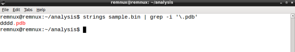
a suspicious string that seems to be related with debug information
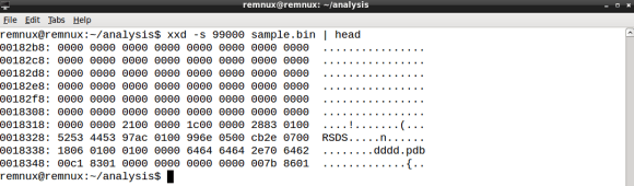
- dddd.pdb
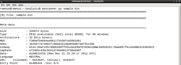
the MD5 hash of the .text section
- 2a7865468f9de73a531f0ce00750ed17
the .rsrc section with high entropy
- .rsrc entropy is 7.98
the symbol GetTickCount import
- Kernel32.dll GetTickCount is present in the IAT
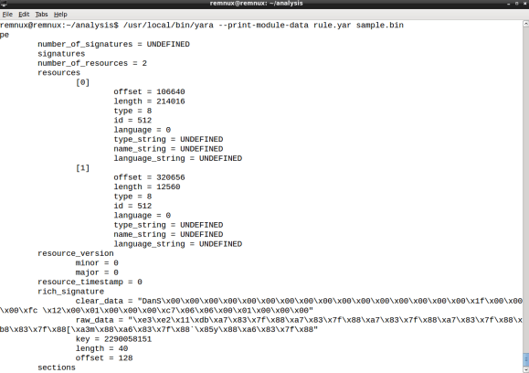
the rich signature XOR key
- 2290058151
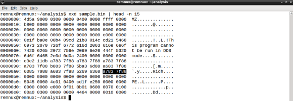
must be a Windows executable file
- 0x4D5A (MZ) found at file offset zero

In part 2 we created a YARA rule file named rule.yar, with the following content:

import "pe"

If you remember the exercise, we needed the PE module in order to parse the sample and extract the Rich signature XOR key. We will use this rule file to develop the remaining code.

The debug information string

In part 1 I have introduced YARA along with the rule format, featuring the strings and condition sections. When you add the dddd.pdb string condition the rule code should be something like:

yara_3_1

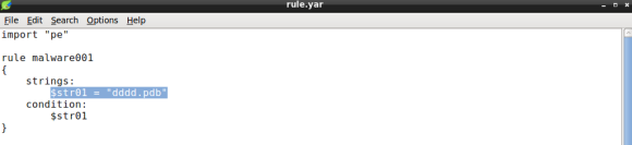
The code above depicts a simple rule object made of a single string variable named $str01 with the value set to the debug string we found.

The section hash condition

Next item to be added to the condition is the .text section hash, using both PE and HASH modules. To do so we will iterate over the PE file sections using two PE module functions: the number_of_sections and sections. The former will be used to iterate over the PE sections, the latter will allow us to fetch section raw_data_offset, or file offset, and raw_data_size, that will be passed as arguments to md5 hash function, in order to compute the md5 hash of the section data:

yara_3_2

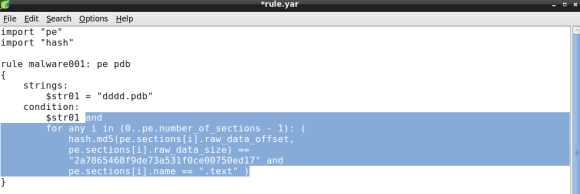
The condition expression now features the for operator comprising two conditions: the section md5 hash and the section name. In essence, YARA will loop through every PE section until it finds a match on the section hash and name.

The resource entropy value

Its now time to add the resource entropy condition. To do so, we will rely on the math module, which will allow us to calculate the entropy of a given size of bytes. Again we will need to iterate over the PE sections using two conditions: the section entropy and the section name (.rsrc):

yara_3_3

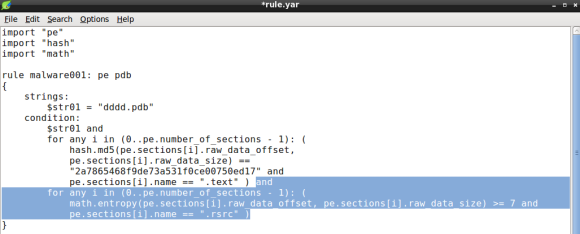
Again we will loop until we find a match, that is a section named .rsrc with entropy above or equal to 7.0. Remember that entropy minimum value is 0.0 and maximum is 8.0, therefore 7.0 is considered high entropy and is frequently associated with packing [1]. Bear in mind that compressed data like images and other types of media can display high entropy, which might result in some false positives [2].

The GetTickCount import

Lets continue improving our YARA rule by adding the GetTickCount import to the condition. For this purpose lets use the PE module imports function that will take two arguments: the library and the DLL name. The GetTickCount function is exported by Kernel32.DLL, so when we passe these arguments to the pe.imports function the rule condition becomes:

yara_3_4

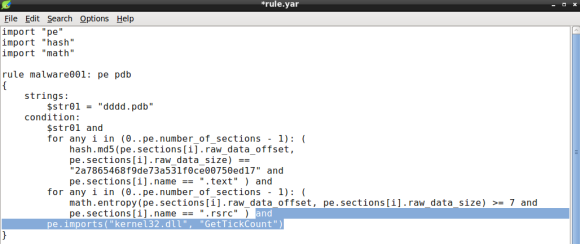
Please note that the DLL name is case insensitive [3].

The XOR key

Our YARA rule is almost complete, we now need to add the rich signature key to the condition. In this particular case the PE module provides the rich_signature function which allow us to match various attributes of the rich signature, in this case the key. The key will be de decimal value of dword used to encode the contents with XOR:

yara_3_5

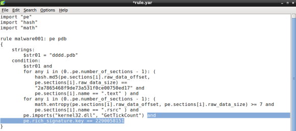
Remember that the XOR key can be obtained either by inspecting the file with a hexdump of the PE header or using YARA PE module parsing capabilities, detailed in part 2 of this series.

The PE file type

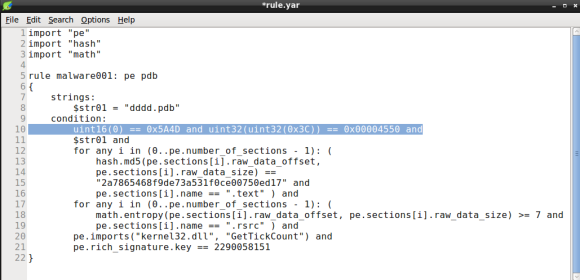
Ok, we are almost done. The last condition will ensure that the file is a portable executable file. In part two of this series we did a quick hex dump of the samples header, which revealed the MZ (ASCII) at file offset zero, a common file signature for PE files. We will use the YARA int## functions to access data at a given position. The int## functions read 8, 16 and 32 bits signed integers, whereas the uint## reads unsigned integers. Both 16 and 32 bits are considered to be little-endian, for big-endian use int##be or uint##be.

Since checking only the first two bytes of the file can lead to false positives we can use a little trick to ensure the file is a PE, by looking for particular PE header values. Specifically we will check for the IMAGE_NT_HEADER Signature member, a dword with value “PE\0\0”. Since the signature file offset is variable we will need to rely on the IMAGE_DOS_HEADER e_lfanew field. e_lfanew value is the 4 byte physical offset of the PE Signature and its located at physical offset 0x3C [4].

With the conditions “MZ” and “PE\0\0” and respective offsets we will use uint16 and uint32 respectively:

yara_3_6

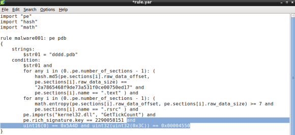
Note how we use the e_lfanew value to pivot the PE Signature, the first uint32 function output, the 0x3C offset, is used as argument in the second uint32 function, which must match the expected value “PE\0\0”.

Conclusion

Ok! We are done, last step is to test the rule against the file using the YARA tool and our brand new rule file rule.yar:

yara_3_7

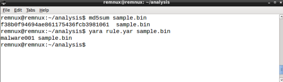
YARA scans the file and, as expected, outputs the rule matched rule ID, in our case malware001.

A final word on YARA performance

While YARA performance might be of little importance if you are scanning a dozen of files, poorly written rules can impact significantly when scanning thousands or millions of files. As a rule of thumb you are advised to avoid using regex statements. Additionally you should ensure that false conditions appear first in the rules condition, this feature is named short-circuit evaluation and it was introduced in YARA 3.4.0 [5]. So how can we improve the rule we just created, in order to leverage YARA performance? In this case we can move the last condition, the PE file check signature, to the top of the statement, by doing so we will avoid checking for the PE header conditions if the file is an executable (i.e. PDF, DOC, etc). Lets see how the new rule looks like:

yara_3_8

If you like to learn more about YARA performance, check the Yara performance guidelines by Florian Roth, as it features lots of tips to keep your YARA rules resource friendly.

References

Structural Entropy Analysis for Automated Malware Classification
Practical Malware Analysis, The Hands-On Guide to Dissecting Malicious Software, Page 283.
YARA Documentation v.3.4.0, PE Module
The Portable Executable File Format
YARA 3.4.0 Release notes

Tagged Malware Analysis, REMnux, Yar

Feb 18 2016

2 Comments

Digital Forensics and Incident Response, Malware Analysis

Unleashing YARA – Part 2

In the first post of this series we uncovered YARA and demonstrated couple of use case that that can be used to justify the integration of this tool throughout the enterprise Incident Response life-cycle. In this post we will step through the requirements for the development of YARA rules specially crafted to match patterns in Windows portable executable “PE” files. Additionally, we will learn how to take advantage of Yara modules in order to create simple but effective rules. Everything will be wrapped-up in a use case where an incident responder, that will be you, will create YARA rules based on the static analysis of a PE file.

Specifically, the use case scenario will be split into two posts. In part 2 we will start with an incident report that will introduce a simple rule development challenge, solely based on static analysis. In the part 3, will cover rule creation, performance tuning and troubleshooting.

Prerequisites

Before we begin you will need a Linux distribution with the following tools:

YARA 3.4.0 (get it here)
pescanner.py (get it here)

If you are in a hurry I advise you to pick REMnux, Lenny Zeltser’s popular Linux distro for malware analysis, which include a generous amount of tools and frameworks used in the dark art of malware analysis and reverse engineering. REMnux is available for download here.

Additionally you will need a piece of malware to analyse, you can get your own copy of the sample from Malwr.com:

Malwr.com report link here

Sample MD5: f38b0f94694ae861175436fcb3981061

WARNING: this is real malware, ensure you will do your analysis in a controlled, isolated and safe environment, like a temporary virtual machine.

Incident Report

Its Wednesday 4:00PM when a incident report notification email drops on your mailbox. It seems that a Network IPS signature was triggered by a suspicious HTTP file download (f38b0f94694ae861175436fcb3981061) hash of a file. You check the details of the IPS alert to see if it stored the sample in a temporary repository for in-depth analysis. You find that the file was successfully stored and its of type PE (executable file), definitely deserves to be look at. After downloading the file you do the usual initial static analysis: Google for the MD5, lookup the hash in Virustotal, analyse the PE header of the file looking for malicious intent. Right of the bat the sample provides a handful of indicators that will help you to understanding how the file will behave during execution. Just what you needed to start developing your own YARA rules.

The challenge

Create a YARA rule that matches the following conditions:

a suspicious string that seems to be related with debug information
the MD5 hash of the .text section
the .rsrc section with high entropy
the symbol GetTickCount import
the rich signature XOR key
must be a Windows executable file

Static Analysis

Before we continue let me write that the details concerning the structure of the PE file are omitted for the sake of brevity. Please see here and here for more information on PE header structure. Onward!

The first challenge is to find a string related with debug information left by the linker [1], specifically we will be looking for a program database file path (i.e. PDB). Lets run the strings command to output the ASCII strings:

strings output

Amid the vast output the dddd.pdb string stands out. This is probably what we are looking for. Note that is important to output the file offset in decimal with -t d suffix so that you can pinpoint the string location within the file structure. If the string is indeed related to debug information it should be part of the RSDS header. Let’s dump a few bytes of the sample using the 99136 offset as a pivot:

xxd output

The presence of RSDS string gives us the confidence to select the string dddd.pdb as the string related to the debug information.

Next we need to compute the hash of the .text section, that typically contains the executable code [2], for this task we will use hiddenillusion’s version of pescanner.py [3] using the sample name as argument:

pescanner.py initial report

pescanner.py report on sections, resources and imports on the PE file

pescanner.py outputs an extensive report about the PE header structure, on which it includes the list of sections along with the hash. Take note of the .text section MD5 hash (2a7865468f9de73a531f0ce00750ed17) as we will need to use it later when creating the YARA rule.

Also in the pescanner.py report we are informed that the .rsrc section as high entropy. This is a suspicious indicator for the presence of heavily obfuscated code. Please keep this in mind when creating the rule, as this info will help us answering the third item in the challenge. Lastly the report also features the list of imported symbols, in which we can see the presence of GetTickCount, a well known anti-debugging timing function [4]. This will be required to answer the fourth entry of the challenge. By the way, the report also mentions the file type, indicating we are in the presence of a PE32 file, which matches the sixth item of the challenge.

Lastly we need to get our hands on the XOR key used to encode the Rich signature, read more about the Rich signature here. You can check existence of this key in two ways: traditionally you would dump the first bytes of the sample, enough to cover all the DOS Header in the PE file, the Rich signature starts at file offset 0x80, and the XOR key will be located in the dword that follows the Rich ASCII string:

yara_2.1_5

Bear in mind that the x86 byte-order is little-endian [5], therefore you need to byte-swap the dword value, so the XOR key value is 0x887f83a7 or 2290058151 in decimal.

Now for the easy way. Remember when I have mentioned in the first post of this series that the YARA scan engine is modular and feature rich? This is because you can use YARA pretty much like pescanner.py, in order to obtain valuable information on the PE header structure. Let’s start by creating the YARA rule file named rule.yar with the following content:

import “pe”

Next execute YARA as follows:

strings command output

By using the –print-module-data argument YARA will output the report of the PE module, on which will include the rich_signature section along with the XOR key decimal value.

Ok, we now have gathered all the info required to start creating the YARA rule and finish the challenge. In the part 3 of this series, we will cover the YARA rule creation process, featuring the information gathered from static analysis. Stay tuned!

References

http://www.godevtool.com/Other/pdb.htm
Practical Malware Analysis: The Hands-On Guide to Dissecting Malicious Software, (page 22)
https://github.com/hiddenillusion/AnalyzePE/blob/master/pescanner.py
http://antukh.com/blog/2015/01/19/malware-techniques-cheat-sheet
http://teaching.idallen.com/cst8281/10w/notes/110_byte_order_endian.html

Tagged Malware Analysis, pescanner.py, REMnux, YARA

Feb 10 2016

Unleashing YARA – Part 1

[Editor’s Note: In the article below, Ricardo Dias who is a SANS GCFA gold certified and a seasoned security professional demonstrates the usefulness of Yara – the Swiss Army knife for Incident Responders. This way you can get familiar with this versatile tool and develop more proactive and mature response practices against threats. ~Luis]

Intro

yara_logo I remember back in 2011 when I’ve first used YARA. I was working as a security analyst on an incident response (IR) team, doing a lot of intrusion detection, forensics and malware analysis. YARA joined the tool set of the team with the purpose to enhance preliminary malware static analysis of portable executable (PE) files. Details from the PE header, imports and strings derived from the analysis resulted in YARA rules and shared within the team. It was considerably faster to check new malware samples against the rule repository when compared to lookup analysis reports. Back then concepts like the kill chain, indicator of compromise (IOC) and threat intelligence where still at its dawn.

In short YARA is an open-source tool capable of searching for strings inside files (1). The tool features a small but powerful command line scanning engine, written in pure C, optimized for speed. The engine is multi-platform, running on Windows, Linux and MacOS X. The tool also features a Python extension providing access to the engine via python scripts. Last but not least the engine is also capable of scanning running processes. YARA rules resemble C code, generally composed of two sections: the strings definition and a, mandatory, boolean expression (condition). Rules can be expressed as shown:

rule evil_executable
{
    strings:
        $ascii_01 = "mozart.pdb"
        $byte_01  = { 44 65 6d 6f 63 72 61 63 79 }
    condition:
        uint16(0) == 0x5A4D and
        1 of ( $ascii_01, $byte_01 )
}

The lexical simplicity of a rule and its boolean logic makes it a perfect IOC. In fact ever since 2011 the number of security vendors supporting YARA rules is increasing, meaning that the tool is no longer limited to the analyst laptop. It is now featured in malware sandboxes, honey-clients, forensic tools and network security appliances (2). Moreover, with the growing security community adopting YARA format to share IOCs, one can easily foresee a wider adoption of the format in the cyber defence arena.

In the meantime YARA became a feature rich scanner, particularly with the integration of modules. In essence modules enable very fine grained scanning while maintaining the rule readability. For example the PE module, specially crafted for handling Windows executable files, one can create a rule that will match a given PE section name. Similarly, the Hash module allows the creation on hashes (i.e. MD5) based on portions of a file, say for example a section of a PE file.

YARA in the incident response team

So how does exactly a tool like YARA integrate in the incident response team? Perhaps the most obvious answer is to develop and use YARA rules when performing malware static analysis, after all this is when the binary file is dissected, disassembled and understood. This gives you the chance to cross-reference the sample with previous analysis, thus saving time in case of a positive match, and creating new rules with the details extracted from the analysis. While there is nothing wrong with this approach, it is still focused on a very specific stage of the incident response. Moreover, if you don’t perform malware analysis you might end up opting to rule out YARA from your tool set.

Lets look at the SPAM analysis use case. If your team analyses suspicious email messages as part of their IR process, there is great chance for you to stumble across documents featuring malicious macros or websites redirecting to exploit kits. A popular tool to analyse suspicious Microsoft Office documents Tools is olevba.py, part of the oletools package (3), it features YARA when parsing OLE embedded objects in order to identify malware campaigns (read more about it here). When dealing with exploit kits, thug (4), a popular low-interaction honey-client that emulates a web browser, also features YARA for exploit kit family identification. In both cases YARA rule interchanging between the IR teams greatly enhances both triage and analysis of SPAM.

Another use case worth mentioning is forensics. Volatility, a popular memory forensics tool, supports YARA scanning (5) in order to pinpoint suspicious artefacts like processes, files, registry keys or mutexes. Traditionally YARA rules created to parse memory file objects benefit from a wider range of observables when compared to a static file rules, which need to deal with packers and cryptors. On the network forensics counterpart, yaraPcap (6), uses YARA for scan network captures (PCAP) files. Like in the SPAM analysis use case, forensic analysts will be in advantage when using YARA rules to leverage the analysis.

Finally, another noteworthy use case is endpoint scanning. That’s right, YARA scanning at the client computer. Since YARA scanning engine is multi-platform, it poses no problems to use Linux developed signatures on a Windows operating system. The only problem one needs to tackle is on how to distribute the scan engine, pull the rules and push the positive matches to a central location. Hipara, a host intrusion prevention system developed in C, is able to perform YARA file based scans and report results back to a central server (7). Another solution would be to develop an executable python script featuring the YARA module along with REST libraries for pull/push operations. The process have been documented, including conceptual code, in the SANS paper “Intelligence-Driven Incident Response with YARA” (read it here). This use case stands as the closing of the circle in IOC development, since it enters the realm of live IR, delivering and important advantage in the identification of advanced threats.

Conclusion

The key point lies in the ability for the IR teams to introduce the procedures for YARA rule creation and use. Tier 1 analysts should be instructed on how to use YARA to enhance incident triage, provide rule feedback, concerning false positives, and fine tuning to Tier 2 analyst. Additionally a repository should be created in order to centralize the rules and ensure the use of up-to-date rules. Last but not least teams should also agree on the rule naming scheme, preferably reflecting the taxonomy used for IR. These are some of the key steps for integrating YARA in the IR process, and to prepare teams for the IOC sharing process.

References:

Tagged Incident Response, Malware Analysis, Threat Intelligence, YARA

Dec 07 2015

4 Comments

Digital Forensics and Incident Response, Incident Handling and Hacker Techniques, Malware Analysis

Malware Analysis – Dridex & Process Hollowing

[In this article we are going to do an analysis of one of the techniques used by the malware authors to hide its malicious intent when executed on Windows operating systems. The technique is not new but is very common across different malware families and is known as process hollowing. We will use OllyDbg to aid our analysis. ~LR]

Lately the threat actors behind Dridex malware have been very active. Across all the recent Dridex phishing campaigns the technique is the same. All the Microsoft Office documents contain embedded macros that download a malicious executable from one of many hard coded URLs. These hard coded URLs normally point to websites owned by legitimate people. The site is compromised in order to store the malicious file and also to hide any attribution related to the threat actors. The encoding and obfuscation techniques used in the macros are constantly changing in order to bypass security controls. The malicious executable also uses encoding, obfuscation and encryption techniques in order to evade antivirus signatures and even sandboxes. This makes AV detection hard. The variants change daily in order to evade the different security products.

When doing malware static analysis of recent samples, it normally does not produce any meaningful results. For example, running the strings command and displaying ASCII and UNICODE strings does not disclose much information about the binary real functionality. This means we might want to run the strings command after the malware has been unpacked. This will produce much more interesting results such as name of functions that interact with network, registry, I/O, etc.

In this case we will look at the following sample:

remnux@remnux:~$ file rudakop.ex_
 rudakop.ex_: PE32 executable for MS Windows (GUI) Intel 80386 32-bit

remnux@remnux:~$ md5sum rudakop.ex_
 6e5654da58c03df6808466f0197207ed  rudakop.ex_

The environment used to do this exercise is the one described in the dynamic malware analysis with RemnuxV5 article. The Virtual Machine that will be used runs Windows XP. First we just run the malware and we can observe it creates a child process with the same name. This can be seen by running the sample and observing Process Explorer from Sysinternals or Process Hacker from Wen Jia Liu. The below picture illustrate this behavior.

This behavior suggests that the malware creates a child process where it extracts an unpacked version of itself.

In this case we will try to unpack this malware sample in order to get more visibility into its functionality. Bottom line, when the packed executable runs it will extract itself into memory and then runs the unpacked code. Before we step into the tools and techniques lets brief review the concept around process hollowing.

This technique, which is similar to the code injection technique, consists in starting a new instance of a legitimate process with the API CreateProcess() with the flag CREATE_SUSPENDED passed as argument. This will execute all the necessary steps in order to create the process and all its structure but will not execute the code.

The suspended state will permit the process address spaced of the legitimate process to be manipulated. More specifically the image base address and its contents.

The manipulations starts by carving out and clearing the virtual address region where the image base of the legitimate process resides. This is achieved using the API NtUnmapViewOfSection().

Then the contents of the malicious code and its image base will be allocated using VirtualAlloc(). During this step the protection attributes for the memory region will be marked as writable and executable. And then the new image is copied over to the carved region using WriteProcessMemory()

Then the main thread, which is still in suspended state, is changed in order to point to the entry point of the new image base using the SetThreadContext() API.

Finally, the ResumeThread() is invoked and the malicious code starts executing.

This technique has been discussed at lengths and is very popular among malware authors. If you want to even go deeper in this concept you can read John Leitch article. Variants of this process exist but the concept is the same. Create a new legitimate process in suspended state, carve its contents, copy the malicious code into the new process and resume execution.

Now lets practice! In order to debug these steps we will use OllyDbg on a virtual machine running Windows XP.

OllyDbg is a powerful, mature and extremely popular debugger for x86 architecture. This amazing tool was created by Olesh Yuschuk. For this exercise we will use version 1.1. The goal is to extract the payload that is used during the process hollowing technique.

When loading this sample into OllyDbg we are presented with two messages. First an error stating “Bad or unknown format of 32bit executable”. OllyDbg can load the executable but it cannot find the entry point (OEP) which suggest the PE headers have been manipulated. Following that the message “compressed code?” is presented. This warning message is normally displayed when the executable is compressed or encrypted. This is a strong indicator that we are dealing with a packed executable. Here we click “No”.

When the sample is loaded we start by creating a breakpoint in CreateProcessW. This is a key step in the process hollowing technique. We do this by clicking in the disassembler window (top left) and then Ctrl+G. Then we write the function name we want to find. When clicking ok this will take us to the memory address of the function. Here we press F2 and a break point is set. The breakpoints can been seen and removed using the menu View – Breakpoints (Alt+B).

Then we start debugging our program by running it. We do this by pressing F9 or menu Debug – Run. Once the break point is reached we can see the moment before CreateProcessW function is invoked and the different arguments that will be loaded into the stack (bottom right). One of the parameters is the CreationFlags where we can see the process is created in suspended mode.

For the sake of brevity we wont perform the breakpoint steps for the other function calls. But the methodology is to set breakpoints across the important function calls. Before we start debugging the program we can set a break point for the different function calls that were mentioned and review how this technique works. In this case we will move into the end of the process hollowing technique were we hit a breakpoint in WriteProcessMemory() . Once the breakpoint is reached we can see the moment before WriteProcessMemory() function is called and the different arguments. In the stack view (bottom right) we can see that one of the parameters is the Buffer. The data stored is this buffer is of particular interest to us because it contains the contents of the malicious code that is going to be written to the legitimate process. In this case might give us the unpacked binary.

Following this step the code is resumed and executed. During the debugging process if we have Process Hacker running in parallel we can see the new process being created. We can also edit its properties and view the memory regions being used and its suspended thread. Finally when the code is resumed we can see the parent process being terminated.

That’s it for today. In the next post we will carve this buffer out and perform further analysis on this sample in order to understand its intent and capabilities.

The threat actors behind malware have many incentives to protect their code. The world of packing , unpacking, debugging and anti-debugging is fascinating. The competition between malware authors and malware analysts is a fierce fight. The malware authors write armored malware in order to evade AV and Sandboxing detection. In addition they go great lengths ensuring the analysis will be difficult. For further reference you may want to look into the following books: Malware Analyst’s Cookbook and DVD: Tools and Techniques for Fighting Malicious Code, the Practical Malware Analysis and Malware Forensics: Investigating and Analyzing Malicious Code . More formal training is available from SANS with GREM course authored by Lenny Zeltser. Free resources are the Dr. FU’s Security blog on Malware analysis tutorials. The Binary Auditing site which contains free IDA Pro training material. Finally, the malware analysis track in the Open Security Training site is awesome. It contains several training videos and material for free!

References:

SANS FOR610: Reverse-Engineering Malware: Malware Analysis Tools and Techniques
Malware Analyst’s Cookbook and DVD: Tools and Techniques for Fighting Malicious Code
http://www.autosectools.com/Process-Hollowing.pdf John Leitch
https://www.trustwave.com/Resources/SpiderLabs-Blog/Analyzing-Malware-Hollow-Processes/
http://journeyintoir.blogspot.ch/2015/02/process-hollowing-meets-cuckoo-sandbox.html

Tagged Debugging malware, Dridex, Malware Analysis, OllyDbg, Process Hollowing, Process Injection

Mar 18 2015

Memory Forensics with Volatility on REMnux v5 – Part 2

Before we continue our hands-on memory forensics exercise, will be good to refresh some concepts on how memory management works on Windows 32 bits operating systems running on x86 architecture. Windows operating systems have a complex and sophisticated memory management system. In particular the way the mapping works between physical and virtual addresses is a great piece of engineering. On 32 bits x86 machines, virtual addresses are 32 bits long which means each process has 4GB of virtual addressable space. In a simplified manner the 4GB of addressable space is divided into two 2GB partitions. One for user mode processes – Low 2GB (0x00000000 through 0x7FFFFFFF) -and another for the Kernel mode – High 2GB (0x80000000 through 0xFFFFFFFF). This default configuration could be changed in the Windows boot configuration data store (BCD) to accommodate 3GB for user mode. When a process is created and a region of virtual address space is allocated – trough VirtualAlloc API – the memory manager creates a VAD (Virtual Address Descriptor) for it. The VAD is essentially a data structure that contains the various elements of the process virtual addresses organized in a balanced tree. Elements such as the base address, access protection, the size of the region, name of mapped files and others are defined on each VAD entry. The Microsoft Windows Internals book goes over in great detail about it.

Fortunately, Brendan Dolan-Gavitt, back in 2007 created a series of plugins for The Volatility Framework to query, walk and perform forensic examinations of the VAD tree. His original paper is available here.

That being said the next step in our quest to find the malicious code. We will use these great plugins to look at the memory ranges that are accessible by the suspicious process virtual address space. This will allows us to look for hidden and injected code. Worth to mention that a great book with excellent resources and exercises about this matter is the Malware Analyst Cookbook from Michael Ligh et. al. Another great resource that also goes into great detailed and was published last year is the Art of Memory Forensics also from Michael Ligh and the Volatility team. Both books mention that among other things the VAD might be useful to find malicious code hiding in another process. Essentially, by looking at the memory ranges that have an access protection marked as executable specially with the PAGE_EXECUTE_READWRITE protection. This suggest that a particular memory range might be concealing executable code. This has been demonstrated by Michael Ligh and was translated into a Volatility plugin named Malfind. This plugin, among other things, detects code that might have been injected into a process address space by looking at its access protections. For this particular case Malfind does not produce results for the explorer.exe (PID 1872). Might be due to the fact that permissions can be applied at a further granularity level than the VAD node level.

Our next hope is to start looking at the different VAD attributes and mapped files of the VAD tree for this suspicious process using the Vadinfo plugin. The Vadinfo plugin goes into great detail displaying info about the process memory and the output might be vast. For the sake of brevity only the first entry is displayed in the following picture.

In this case the output of the Vadinfo plugin displays almost two hundred VAD nodes and its details. Because we are looking for specific IOCs that we found we want to further look into these memory regions. This is where the Vaddump plugin comes to great help. Vaddump is able to carve our each memory range specified on the VAD node and dump the data into a file.

Then we can do some command line kung-fu to look into those files. We can determine what kind of files we have in the folder and also look for the indicators we found previously when performing dynamic analysis. In this case we could observe that the string “topic.php” appears in five different occasions using the default strings command. In addition it appears once when running strings with a different encoding criteria – and this exactly matches the found IOC.

On a side note is interesting to see based on the file names the memory ranges that span the virtual address space from 0x00000000 to 0x7FFFFFFF. And you also could see that there is some groups of addresses more contiguous than others. This related on how the process memory layout looks like. The following image illustrates this layout on a x86 32bit Windows machine. This can be further visualized using VMMap tool from Mark Russinovich and available on the Sysinternals Suite.

Back to our analysis, one first step is to look across dumped data from the Vaddump plugin see if there is any interesting executables files. We observed that the previous search found several Windows PE32 files. Running again our loop to look for Windows PE32 files we see that it contains 81 executables. However, we also know the majority of them are DLL’s. Lets scan trough the files to determine which ones are not DLL’s. This gives good results because only two files matched our search.

Based on the two previous results we run again the Vadinfo plugin and looked deeper into those specific memory regions. The first memory region which starts at 0x01000000 contains normal attributes and a mapped file that matches the process name. The second memory regions which starts at 0x00090000 is more interesting. Specially the node has the tag VadS. According to Michael Ligh and the Volatility Team this type of memory regions are strong candidates to have injected code.

Next step? run strings into this memory region to see what comes up and don’t forget to run strings with a different encoding criteria.

As you could see below, on the left side, we have a small set of the strings found on the memory region. This information gives great insight into the malware capabilities, gives further hints that can be used to identify the malware on other systems and can further help our analysis. On the right side you have a subset of the strings found using a different encoding criteria. This goes together with previous strings and gives you even further insight into what the malware does, its capabilities and the worst it can do.

Security incident handlers might be satisfied with dynamic analysis performed on the malware because they can extract IOCs that might be used to identify the malware across the defense systems and aid the incident response actions. However, trough this exercise we gained intelligence about what the malware does by performing memory forensics. In addition, as malware evolves and avoids footprints in the hard drive the memory analysis will be needed to further understand the malware capabilities. This allows us to augment prevention controls and improve detection and response actions. Nonetheless, one might want to even go further deep and not only determine what the malware does but also how. That being said the next logical step would be to get the unpacked malware from memory and perform static analysis on the sample. Once again, Volatility Framework offers the capability of extracting PE files from memory. Then they can be loaded into a dissasembler and/or a debugger. To extract these files from memory there are a variety of plugins. We will use the dlldump plugin because it allows you to extract PE files from hidden or injected memory regions.

There are some caveats with the PE extraction plugins and there is a new sport around malware writers on how to manipulate PE files in memory or scramble the different sections so the malware analysts have a tougher time getting them. The Art of Memory Forensics and the The Rootkit Arsenal book goes into great detail into those aspects.

With the malware sample unpacked and extracted from memory we can now go in and perform static analysis … this is left for another post.

That’s it – During the first part we defined the steps needed to acquire the RAM data for a VMware virtual machine before and after infection. Then, we started our quest of malware hunting in memory. We did this by benchmarking both memory captures against each other and by applying the intelligence gained during the dynamic analysis. On the second part we went deeper into the fascinating world of memory forensics. We manage to find the injected malware in memory that was hidden in a VAD entry of the explorer.exe process address space. We got great intel about the malware capabilities by looking at strings on memory regions and finally we extracted the hidden PE file. All this was performed using the incredible Volatility Framework that does a superb job removing all the complex memory details from the investigation.

Malware sample used in this exercise:

remnux@remnux:~/Desktop$ pehash torrentlocker.exe
file:             torrentlocker.exe
md5:              4cbeb9cd18604fd16d1fa4c4350d8ab0
sha1:             eaa4b62ef92e9413477728325be004a5a43d4c83
ssdeep:           6144:NZ3RRJKEj8Emqh9ijN9MMd30zW73KQgpc837NBH:LhRzwEm7jEjz+/g2o7fH

References:

Ligh, M. H., Case, A., Levy, J., & Walters, A. (2014). Art of memory forensics: Detecting malware and threats in Windows, Linux, and Mac memory
Ligh, M. H. (2011). Malware analyst’s cookbook and DVD: Tools and techniques for fighting malicious code.
Russinovich, M. E., Solomon, D. A., & Ionescu, A. (2012). Windows internals: Part 1
Russinovich, M. E., Solomon, D. A., & Ionescu, A. (2012). Windows internals: Part 2
Blunden, B. (2009). The rootkit arsenal: Escape and evasion in the dark corners of the system.
Zeltser, Lenny (2013) SANS FOR610: Reverse-Engineering Malware: Malware Analysis Tools and Techniques

Tagged Finding injected code into memory, Malware Analysis, Memory Forensics, Michael Ligh, REMnux, VAD Tree, virtual address space, Volatility Framework

Mar 16 2015

3 Comments

Digital Forensics and Incident Response, Malware Analysis

Memory Forensics with Volatility on REMnux v5 – Part 1

As threats and technology continue to evolve and malware becomes more sophisticated, the acquisition of volatility data and its forensic analysis is a key step during incident response and digital forensics. This article is about acquiring RAM from a disposable virtual machine before and after malware infection. This data will then be analyzed using the powerful Volatility Framework. The steps described here go hand in hand with the steps described on previous blog posts here and here about dynamic malware analysis.

We will use the methodology stated in previous post. We will start the virtual machine in a known clean state by restoring it from a snapshot or starting a golden copy. Then we will suspend/pause the machine in order to create a checkpoint state file. This operation will create a VMSS file inside the directory where the virtual machine is stored. Then we will use a tool provided by VMware named Vmss2core to convert this VMSS file into a WinDbg file (memory.dmp). From VMware website: Vmss2core is a tool to convert VMware checkpoint state files into formats that third party debugger tools understand. Last version is available here. It can handle both suspend (.vmss) and snapshot (.vmsn) checkpoint state files as well as both monolithic and non-monolithic (separate .vmem file) encapsulation of checkpoint state data. This tools will allow us to convert the VMware memory file into a format that is readable by the Volatility Framework.

Next, we restore the virtual machine to back where it was and we infect it with malware. After that, we suspend the machine again and repeat the previous steps. This allow us to have two memory dumps that we can compare against each other in order to facilitate the finding of malicious code.

To perform the analysis and the memory forensics we will use the powerful Volatility Framework. The Volatility Framework born based on the research that was done by AAron Walters and Nick Petroni on Volatools and FATkit. The first release of the Volatility Framework was released in 2007. In 2008 the volatility team won the DFRWS and added the features used in the challenge to Volatility 1.3. Seven years have passed and this framework has gained a lot of popularity and attention from the security community. The outcome has been a very powerful, modular and feature rich framework that combines a number of tools to perform memory forensics. The framework is written in Python and allows plugins to be easily added in order to add features. Nowadays it is on version 2.4, it supports a variety of operating systems and is being actively maintained.

Below the steps needed to acquire the RAM data for a VMware virtual machine:

Restore the VMware snapshot to a known clean state.
Pause the Virtual Machine
Execute vmss2core_win.exe
Rename the memory.dmp file to memory-before.dmp
Resume the virtual machine
Execute the malware
Pause the virtual machine
Execute vmss2core_win.exe
Rename the memory.dmp file to memory-after.dmp

The following picture ilustrates the usage of Vmss2core_win.exe.

After performing this steps we can proceed to the analysis. First we move the memory dumps to REMnux. Then we start the Volatility Framework which comes pre-installed. We start our analysis by listing the process as a tree using the “pstree” module on both the clean and infected memory image. With this we can benchmark the infected machine and easily spot difference on infections performed by commodity malware. In this case we can easily spot that on the infected machine there a process named explorer.exe (PID 1872) that references a parent process (PPID 1380) that is not listed. In addition we can observe the processes vssadmin.exe (PID 1168) and iexplorer.exe (PID 1224) which were spawned by explorer.exe. Vsadmin.exe can manage volume shadow copies on the system. This strongly suggests that we are in presence of something suspicious.

Next step is to do a deep dive. During the previous dynamic malware analysis articles series were we analyzed the same piece of malware we were able to extract indicators of compromise (IOC). These IOC’s were extracted from our analysis performed at the network level and system level. We will use this information for our own advantage in order to reduce the effort needed to find Evil. We knew that after the infection the malware will attempt to contact the C&C using a HTTP POST request to the URL topic.php which was hosted in Russia.

Let’s use this pieces of information to search and identify the malicious code. To perform this we will look for ASCII and UNICODE strings that match those artifacts using src_strings utility that is part of The Sleuth Kit from Brian Carrier and is installed on REMnux.

The parameter “-t d” will tell the tool to print the location of the string in decimal. We save this findings in a text file. The results are then used by Volatility. Next, we invoke Volatility and use the “strings” plugin that can map physical offsets to virtual addresses – this only works on raw memory images and not on crash dumps – . It works by traversing all the active processes and is able to determine which ones accessed the specified strings. In case of a match we will have a good hint on where the malicious code might reside. In this case the plugin is able to match the strings with the process ID 1872 on two different virtual addresses. This corroborates the fact that on the previous step we saw this process without a parent process which was rather suspicions . Another clue that we might be in good direction.

This can be easily confirmed by listing the process ID 1872 using the “pslist” module. Given this fact we proceed with the extract of this process from memory to a file using the “procmemdump” plugin. Volatility Framework is so powerful that it can parse PE headers in memory and carve them out. With this plugin we can dump the process executable using its PID. After extraction we can verify that the file commands correctly identifies the file as a PE32 executable. Then we can verify that the string we found previous is indeed part of this process.

Well, looks like the string “topic.php” is not in the data we just extracted. However, as we could see in the previous analysis steps we determined that the actions performed by the malicious code were in the context of this process. Furthermore, during the basic static analysis performed (see previous post) on the malicious executable we saw that it references very few libraries but two of them were noteworthy. The LoadLibrary and GetProcAddress. This suggest the malicious executable was either packed or encrypted. In addition those libraries suggest that malicious code was injected into a process. There are several techniques used by threat actors to inject malicious code into benign processes. I will expand on this techniques on a different blog post. As conclusion we might be looking at malicious code that was injected in the process explorer.exe (PID 1832) and is somehow concealed. This means we will need to look deeper into the obscure and fascinating world of memory forensics. Part two will follow!

Malware sample used in this exercise:

remnux@remnux:~/Desktop$ pehash torrentlocker.exe
file:             torrentlocker.exe
md5:              4cbeb9cd18604fd16d1fa4c4350d8ab0
sha1:             eaa4b62ef92e9413477728325be004a5a43d4c83
ssdeep:           6144:NZ3RRJKEj8Emqh9ijN9MMd30zW73KQgpc837NBH:LhRzwEm7jEjz+/g2o7fH

References:

Ligh, M. H. (2011). Malware analyst’s cookbook and DVD: Tools and techniques for fighting malicious code.
Zeltser, Lenny (2013) SANS FOR610: Reverse-Engineering Malware: Malware Analysis Tools and Techniques

Tagged Acquire Memory from Virtual Machine, malicious code, Malware Analysis, Memory Forensics, Volatility Framework

Jan 21 2015

2 Comments

Digital Forensics and Incident Response, Malware Analysis

Dynamic Malware Analysis with REMnux v5 – Part 2

During part one we created the environment to perform dynamic malware analysis with REMnux toolkit. Then the malware was executed and all the interactions with the network were observed and captured. Essentially, the malware was executed in a disposable virtual machine and all the traffic – including SSL – was intercepted.

Now, to further acquire information that would help us answering the questions made during part 1, it would be relevant to observe what happens at the system level.

Below recipe involves running Process Monitor from Sysinternals. Process Monitor is an advanced monitoring tool for Windows that shows real-time file system, Registry and process/thread activity, In parallel we run a packet capture with Wireshark on the disposable machine or we run tcpdump on REMnux. These tools will be started before malware executed and stopped moments after the infection. Then we will import this data – pcap and procmon – into ProcDOT. ProcDOT is a free tool created by Christian Wojne from CERT.at. It runs on Windows or Linux and is installed on REMNux This tool has the capability to parse the Procmon data. Then correlates it with the pcap and transforms the data into a picture. This enables malware visual analysis. This method can be of great help for a effective and efficient dynamic malware analysis. The steps using part 1 model are:

Restore the VMware snapshot.
Start Process Monitor (need to be installed beforehand) and configure Columns fields to be compatible with ProcDOT.
Start Wireshark or tcpdump on REMnux and start capturing traffic.
Copy the malware to the virtual machine and run the malware.
Stop the wireshark capture and export the traffic into PCAP.
Stop the Process Monitor capture and export the results into CSV.
Move the PCAP and CSV file to REMnux.
Power off the infected machine.
Execute ProcDOT and import the procmon and pcap data.
Select the process and render the analysis.
Run trough the animation to understand the timing aspects.

The picture below demonstrate the result (for the sake of size elements such of registry key and paths have been removed):

This visualization technique is very helpful in order to determine in a very quick way what the malware does. The graph produced by ProcDOT is interactive and you can play an animation of it in order to determine in which sequence the events occurred. In this case several relevant events happened. You can easily observe that:

The executable torrentlocker.exe starts execution and invokes a new thread id 1924
The thread id 1924 creates a new suspicious file named 01000000
Thread id 1924 creates a new process named “explorer.exe” with pid 1928
This new process creates several actions including
A suspicious executable file is created under c:\windows named izigajev.exe
A new AutoStart registry key is created invoking the just created executable file
The file Administrator.wab is read and data written to it.
A new process name vssadmin.exe is invoked

By looking at this sequence of events we can conclude that the malware performs process injection by injecting its malicious code into a benign process. Creates a copy of itself and drops it into Windows folder. Maintains persistence by adding the dropped executable into the auto start registry key and creates several suspicious files.

A very simple, fast and effective method that can speed up the malware analysis. Using this visual analytic technique and the one described on part one you can gather indicators that could now be used to identify the malware in motion (network) or at rest (file system/registry) across your network. Further they could be used to augment existing security controls and find additional infected systems.

Tagged Dynamic Malware Analysis, Malware Analysis, Malware visualization, ProcDOT, REMnux

Count Upon Security

Increase security awareness. Promote, reinforce and learn security skills.

Tag Archives: Malware Analysis

Unleashing YARA – Part 3

The section hash condition

The resource entropy value

The GetTickCount import

The XOR key

The PE file type

Conclusion

A final word on YARA performance

References

Unleashing YARA – Part 2

Prerequisites

Incident Report

The challenge

Static Analysis

References

Unleashing YARA – Part 1

Intro

YARA in the incident response team

Conclusion

Malware Analysis – Dridex & Process Hollowing

Memory Forensics with Volatility on REMnux v5 – Part 2

Memory Forensics with Volatility on REMnux v5 – Part 1

Dynamic Malware Analysis with REMnux v5 – Part 2